L’ensemble \mathbb{Z}

Contenu

L’ensemble \(\mathbb{Z}\)#

Les nombres négatifs sont apparus comme des fantômes, mais ils se sont révélés être les plus fidèles compagnons des mathématiques.

John Napier

Construction de \(\mathbb{Z}\)#

L’équation \(x + n = m\) n’a de solution dans \(\mathbb{N}\) que si \(n \leq m\). Pour remédier à cela, on construit \(\mathbb{Z}\) comme un ensemble quotient.

Définition 45 (Relation d’équivalence sur \(\mathbb{N}^2\))

On définit sur \(\mathbb{N}^2\) : \((a, b) \sim (c, d) \iff a + d = b + c\)

(intuition : \((a, b)\) représente la différence \(a - b\)).

Proposition 44

\(\sim\) est une relation d’équivalence. L’ensemble \(\mathbb{Z} = \mathbb{N}^2/{\sim}\) est un anneau commutatif intègre, et \((\mathbb{Z}, +, \cdot)\) vérifie :

\((a,b) + (c,d) = (a+c, b+d)\), d’élément neutre \(\overline{(0,0)}\)
\((a,b) \cdot (c,d) = (ac+bd, ad+bc)\), d’élément neutre \(\overline{(1,0)}\)
\(-\overline{(a,b)} = \overline{(b,a)}\)

Remarque 21

On identifie \(\mathbb{N}\) à son image \(n \mapsto \overline{(n,0)}\) dans \(\mathbb{Z}\), et on note \(\overline{(0,n)} = -n\). Tout entier relatif s’écrit de façon unique comme \(n\) ou \(-n\) avec \(n \in \mathbb{N}\).

Structure de \(\mathbb{Z}\)#

Proposition 45 (\((\mathbb{Z}, +, \cdot)\) est un anneau commutatif intègre)

Groupe abélien \((\mathbb{Z}, +)\) : neutre \(0\), inverse \(-n\).
Monoïde commutatif \((\mathbb{Z}, \cdot)\) : neutre \(1\).
Intégrité : \(ab = 0 \implies a = 0\) ou \(b = 0\).
Non corps : \(2\) n’est pas inversible dans \(\mathbb{Z}\).

Valeur absolue et ordre#

Définition 46 (Valeur absolue et ordre)

\(|n| = n\) si \(n \geq 0\), \(|n| = -n\) si \(n < 0\).

\(m \leq n \iff n - m \in \mathbb{N}\).

Proposition 46 (Propriétés)

\(|mn| = |m| \cdot |n|\)
\(|m + n| \leq |m| + |n|\) (inégalité triangulaire)
\(\big||m| - |n|\big| \leq |m - n|\) (inégalité triangulaire inverse)
\((\mathbb{Z}, \leq)\) est un ordre total, mais pas bien fondé (\(\mathbb{Z}\) n’a pas de minimum).

Proof. Inégalité triangulaire : \(-|m| \leq m \leq |m|\) et \(-|n| \leq n \leq |n|\), donc \(-(|m|+|n|) \leq m+n \leq |m|+|n|\).

Division euclidienne dans \(\mathbb{Z}\)#

Proposition 47 (Division euclidienne dans \(\mathbb{Z}\))

Pour tout \(a \in \mathbb{Z}\) et \(b \in \mathbb{Z}^*\), il existe un unique \((q, r) \in \mathbb{Z} \times \mathbb{N}\) tel que

\[a = bq + r \quad \text{et} \quad 0 \leq r < |b|\]

Identité de Bézout et algorithme d’Euclide étendu#

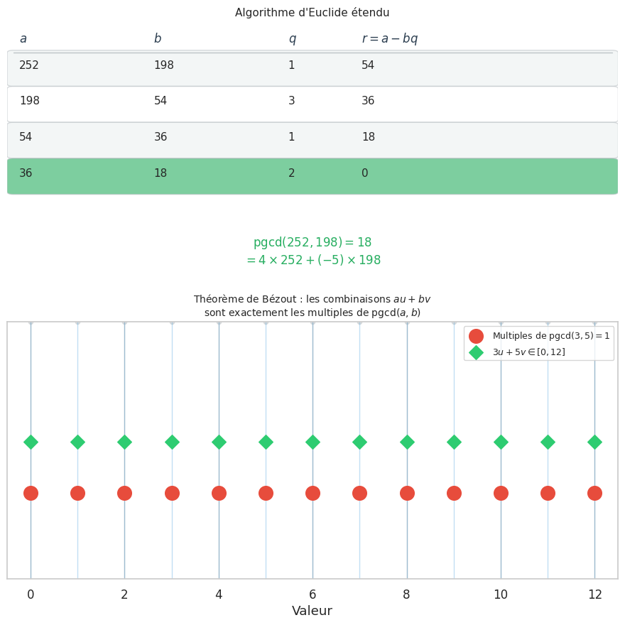
Proposition 48 (Théorème de Bézout)

Pour tous \(a, b \in \mathbb{Z}\) (non tous deux nuls), il existe \(u, v \in \mathbb{Z}\) tels que

\[au + bv = \pgcd(a, b)\]

Proof. L’ensemble \(\{au + bv \mid u, v \in \mathbb{Z}\}\) est un sous-groupe de \((\mathbb{Z}, +)\), donc de la forme \(d\mathbb{Z}\) pour un certain \(d \geq 0\) (cf. chapitre 3). On vérifie que \(d = \pgcd(a, b)\) :

\(d \mid a\) et \(d \mid b\) (car \(a = a \cdot 1 + b \cdot 0\) et \(b \in d\mathbb{Z}\), donc \(d \mid a\)).
Si \(e \mid a\) et \(e \mid b\), alors \(e \mid (au + bv) = d\), donc \(e \leq d\). Ainsi \(d\) est bien le pgcd.

Proposition 49 (Algorithme d’Euclide étendu)

La remontée de l’algorithme d’Euclide fournit explicitement \(u\) et \(v\) tels que \(au + bv = \pgcd(a,b)\).

Exemple 19

\(\pgcd(252, 198)\) :

\[252 = 198 \cdot 1 + 54 \implies 54 = 252 - 198 \cdot 1\]

\[198 = 54 \cdot 3 + 36 \implies 36 = 198 - 54 \cdot 3\]

\[54 = 36 \cdot 1 + 18 \implies 18 = 54 - 36 \cdot 1\]

\[36 = 18 \cdot 2 + 0\]

Remontée : \(18 = 54 - 36 = 54 - (198 - 54 \cdot 3) = 4 \cdot 54 - 198 = 4(252 - 198) - 198 = 4 \cdot 252 - 5 \cdot 198\).

Donc \(\pgcd(252, 198) = 18\) avec \(u = 4\), \(v = -5\).

Proposition 50 (Lemme de Gauss)

Si \(a \mid bc\) et \(\pgcd(a, b) = 1\), alors \(a \mid c\).

Proof. Par Bézout, \(\exists u, v,\ au + bv = 1\). Multiplier par \(c\) : \(auc + bvc = c\). Comme \(a \mid auc\) et \(a \mid bc\) donc \(a \mid bvc\), on a \(a \mid c\).

Proposition 51 (Lemme d’Euclide)

Si \(p\) est premier et \(p \mid ab\), alors \(p \mid a\) ou \(p \mid b\).

Proof. Si \(p \nmid a\), alors \(\pgcd(p, a) = 1\) (car les seuls diviseurs de \(p\) sont \(1\) et \(p\)). Par le lemme de Gauss, \(p \mid b\).

_images/3d7dd046fb660ba36587b5a850968426c35a04d848811395f9582557e485b715.png

Congruences et arithmétique modulaire#

Définition 47 (Congruence)

Pour \(n \in \mathbb{N}^*\), on dit que \(a \equiv b [n]\) (« \(a\) est congru à \(b\) modulo \(n\) ») si \(n \mid (a - b)\).

Proposition 52 (Propriétés des congruences)

La congruence modulo \(n\) est une relation d’équivalence sur \(\mathbb{Z}\), compatible avec \(+\) et \(\cdot\) :

\[a \equiv a' [n] \land b \equiv b' [n] \implies a+b \equiv a'+b' [n] \land ab \equiv a'b' [n]\]

Définition 48 (Anneau \(\mathbb{Z}/n\mathbb{Z}\))

L’ensemble des classes de congruence modulo \(n\), noté \(\mathbb{Z}/n\mathbb{Z} = \{\bar{0}, \bar{1}, \ldots, \overline{n-1}\}\), est un anneau commutatif pour \(\bar{a} + \bar{b} = \overline{a+b}\) et \(\bar{a} \cdot \bar{b} = \overline{ab}\).

Proposition 53 (\(\mathbb{Z}/n\mathbb{Z}\) est un corps \(\iff\) \(n\) est premier)

Plus précisément : \(\bar{a}\) est inversible dans \(\mathbb{Z}/n\mathbb{Z}\) si et seulement si \(\pgcd(a, n) = 1\).

Proof. \(\bar{a}\) inversible \(\iff \exists \bar{u},\ \bar{a}\bar{u} = \bar{1} \iff \exists u, v \in \mathbb{Z},\ au + nv = 1 \iff \pgcd(a, n) = 1\) (Bézout).

Définition 49 (Groupe des inversibles)

Le groupe des unités de \(\mathbb{Z}/n\mathbb{Z}\) est \((\mathbb{Z}/n\mathbb{Z})^* = \{\bar{a} \mid \pgcd(a, n) = 1\}\).

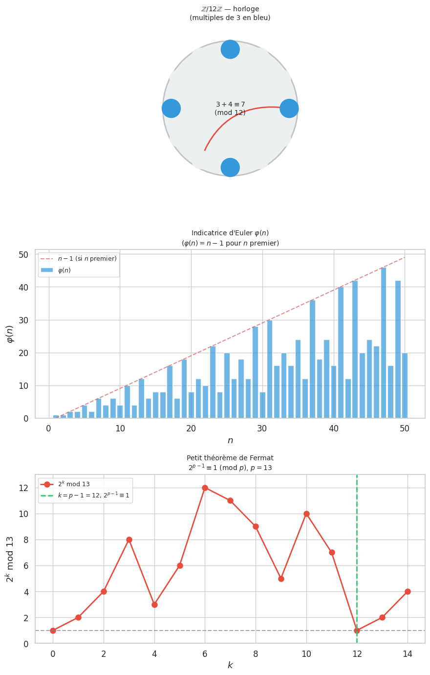
Définition 50 (Indicatrice d’Euler)

\(\varphi(n) = \#\{k \in \{1, \ldots, n\} \mid \pgcd(k, n) = 1\} = |(\mathbb{Z}/n\mathbb{Z})^*|\)

Proposition 54 (Formule de l’indicatrice d’Euler)

\[\varphi(n) = n \prod_{p \mid n,\ p\ \text{premier}} \left(1 - \frac{1}{p}\right)\]

Proof. Par inclusion-exclusion. Si \(n = p_1^{\alpha_1} \cdots p_k^{\alpha_k}\), les entiers \(\leq n\) non copremiers avec \(n\) sont ceux divisibles par au moins un \(p_i\). Par inclusion-exclusion :

\[\varphi(n) = n\left(1 - \frac{1}{p_1}\right)\left(1 - \frac{1}{p_2}\right)\cdots\left(1 - \frac{1}{p_k}\right)\]

Proposition 55 (Théorème d’Euler et petit théorème de Fermat)

Euler : Pour \(\pgcd(a, n) = 1\) : \(a^{\varphi(n)} \equiv 1 [n]\).
Fermat : Pour \(p\) premier et \(p \nmid a\) : \(a^{p-1} \equiv 1 [p]\).

Proof. Le groupe \((\mathbb{Z}/n\mathbb{Z})^*\) est d’ordre \(\varphi(n)\). Par le théorème de Lagrange (ordre d’un élément divise l’ordre du groupe), \(\bar{a}^{\varphi(n)} = \bar{1}\).

Le cas de Fermat est le cas particulier \(n = p\) premier, où \(\varphi(p) = p - 1\).

Exemple 20

\(a = 7\), \(n = 10\) : \(\varphi(10) = \varphi(2)\varphi(5) = 1 \cdot 4 = 4\). Donc \(7^4 \equiv 1 [10]\). En effet, \(7^2 = 49 \equiv 9\), \(7^4 \equiv 81 \equiv 1 [10]\). ✓

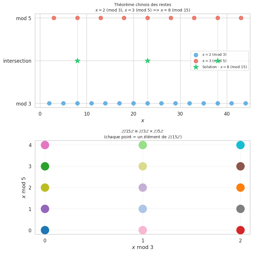
Théorème chinois des restes#

Proposition 56 (Théorème chinois des restes (CRT))

Soient \(n_1, \ldots, n_k \in \mathbb{N}^*\) deux à deux copremiers. Pour tous \(a_1, \ldots, a_k \in \mathbb{Z}\), le système

\[x \equiv a_i [n_i], \quad i = 1, \ldots, k\]

admet une unique solution modulo \(N = n_1 \cdots n_k\).

Proof. Pour \(k = 2\) : comme \(\pgcd(n_1, n_2) = 1\), Bézout donne \(u_1 n_1 + u_2 n_2 = 1\). Posons \(x = a_1 u_2 n_2 + a_2 u_1 n_1\). Alors \(x \equiv a_1 \cdot 1 \equiv a_1 [n_1]\) et \(x \equiv a_2 \cdot 1 \equiv a_2 [n_2]\). L’unicité modulo \(N = n_1 n_2\) découle de \(n_1 \mid x\) et \(n_2 \mid x \implies n_1 n_2 \mid x\) (copremiers).

Le cas général se démontre par récurrence.

Remarque 22

Le CRT est isomorphe à l’anneau : \(\mathbb{Z}/N\mathbb{Z} \cong \mathbb{Z}/n_1\mathbb{Z} \times \cdots \times \mathbb{Z}/n_k\mathbb{Z}\) (isomorphisme d’anneaux). Il est fondamental en cryptographie (RSA), en algèbre computationnelle (FFT), et en théorie des nombres.

_images/f756c4831e7c45e665bd274dcb5017ef6e63e661b9507554c4db21e9a9e1f87b.png

Show code cell source

Hide code cell source

# Théorème chinois des restes : visualisation
fig, axes = plt.subplots(2, 1, figsize=(9, 9))

# CRT : x ≡ 2 (mod 3), x ≡ 3 (mod 5)  => x ≡ 8 (mod 15)
n1, a1 = 3, 2
n2, a2 = 5, 3
N = n1 * n2

solutions = [x for x in range(N) if x % n1 == a1 and x % n2 == a2]
print(f"Solution : {solutions[0]} mod {N}")

ax = axes[0]
x_range = range(3 * N)
class1 = [x for x in x_range if x % n1 == a1]
class2 = [x for x in x_range if x % n2 == a2]
intersect = [x for x in x_range if x % n1 == a1 and x % n2 == a2]

ax.scatter(class1, [1]*len(class1), s=100, color='#3498db', alpha=0.7,
           label=f'$x = {a1}$ (mod {n1})', zorder=5)
ax.scatter(class2, [2]*len(class2), s=100, color='#e74c3c', alpha=0.7,
           label=f'$x = {a2}$ (mod {n2})', zorder=5)
ax.scatter(intersect, [1.5]*len(intersect), s=200, color='#2ecc71',
           marker='*', label=f'Solution : $x = {solutions[0]}$ (mod {N})', zorder=6)

for x_sol in intersect:
    ax.axvline(x=x_sol, color='#2ecc71', alpha=0.3, lw=1)

ax.set_xlim(-1, 3*N)
ax.set_yticks([1, 1.5, 2])
ax.set_yticklabels([f'mod {n1}', 'intersection', f'mod {n2}'])
ax.set_xlabel('$x$')
ax.set_title(f'Théorème chinois des restes\n$x = {a1}$ (mod {n1}), $x = {a2}$ (mod {n2}) => $x = {solutions[0]}$ (mod {N})',
             fontsize=10)
ax.legend(fontsize=9)

# Isomorphisme CRT : Z/15Z ≅ Z/3Z × Z/5Z
ax2 = axes[1]
pairs = [(x % 3, x % 5) for x in range(15)]
from matplotlib.collections import LineCollection

for x, (r3, r5) in enumerate(pairs):
    color = plt.cm.tab20(x / 15)
    ax2.scatter([r3], [r5], s=400, color=color, zorder=5)
    ax2.text(r3, r5, str(x), ha='center', va='center', fontsize=9, color='white', fontweight='bold')

ax2.set_xlabel('$x$ mod 3'); ax2.set_ylabel('$x$ mod 5')
ax2.set_xticks([0, 1, 2]); ax2.set_yticks([0, 1, 2, 3, 4])
ax2.set_title('$\\mathbb{Z}/15\\mathbb{Z} \\cong \\mathbb{Z}/3\\mathbb{Z} \\times \\mathbb{Z}/5\\mathbb{Z}$\n(chaque point = un élément de $\\mathbb{Z}/15\\mathbb{Z}$)', fontsize=10)
ax2.grid(True, alpha=0.3)

plt.tight_layout()
plt.show()

Solution : 8 mod 15

_images/8963371631292e7b85120f81ce54e1b5b4f310762eafe57504338e722dcb301b.png

Nombres premiers et cryptographie#

Remarque 23

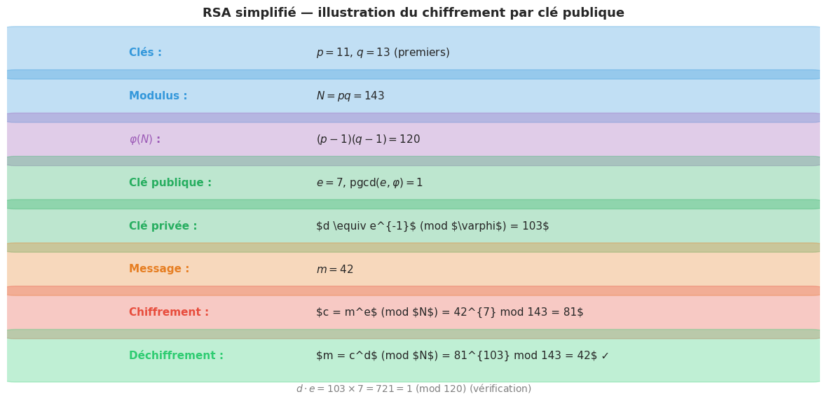
Le chiffrement RSA repose sur les structures vues ici :

On choisit deux grands premiers \(p\) et \(q\), pose \(N = pq\).
L’exposant public \(e\) vérifie \(\pgcd(e, \varphi(N)) = 1\) où \(\varphi(N) = (p-1)(q-1)\).
L’exposant privé \(d\) est l’inverse de \(e\) modulo \(\varphi(N)\) : \(de \equiv 1 [\varphi(N)]\).
Chiffrement : \(c \equiv m^e [N]\). Déchiffrement : \(m \equiv c^d [N]\) (par Euler : \(c^d = m^{ed} = m^{1 + k\varphi(N)} \equiv m\)).

La sécurité repose sur la difficulté de factoriser \(N\) pour trouver \(p\) et \(q\).

_images/6f5302c93b5d46ed7d4908ac4f581d4a83ac00dffba6c71b0a398ebee037de17.png