Espaces préhilbertiens

La notion de produit scalaire est à la géométrie ce que la notion de mesure est à l’analyse : elle permet de quantifier.

John von Neumann

Introduction

Le chapitre précédent a développé la théorie générale des formes bilinéaires. Nous nous concentrons ici sur le cas le plus riche : les formes bilinéaires symétriques définies positives, c’est-à-dire les produits scalaires. Ce cadre fournit les notions de norme, d’angle, de projection orthogonale, d’adjoint, et culmine avec le théorème spectral : toute matrice symétrique réelle est diagonalisable en base orthonormale.

Show code cell source

Hide code cell source

import numpy as np
import matplotlib.pyplot as plt
from matplotlib.patches import FancyArrowPatch, Arc
import matplotlib.patches as mpatches

fig, axes = plt.subplots(3, 1, figsize=(9, 14))

# --- Produit scalaire : angle et norme ---
ax = axes[0]
u = np.array([2.0, 1.0])
v = np.array([0.5, 2.0])
dot = np.dot(u, v)
nu = np.linalg.norm(u); nv = np.linalg.norm(v)
angle = np.arccos(dot/(nu*nv))

ax.annotate('', xy=u, xytext=(0,0),
            arrowprops=dict(arrowstyle='->', color='blue', lw=2))
ax.annotate('', xy=v, xytext=(0,0),
            arrowprops=dict(arrowstyle='->', color='red', lw=2))
ax.text(u[0]+0.1, u[1]+0.05, '$u$', fontsize=13, color='blue')
ax.text(v[0]+0.1, v[1]+0.05, '$v$', fontsize=13, color='red')

arc = Arc((0,0), 0.8, 0.8, angle=0,
          theta1=np.degrees(np.arctan2(u[1],u[0])),
          theta2=np.degrees(np.arctan2(v[1],v[0])), color='green', lw=2)
ax.add_patch(arc)
mid_angle = (np.arctan2(u[1],u[0]) + np.arctan2(v[1],v[0]))/2
ax.text(0.5*np.cos(mid_angle), 0.5*np.sin(mid_angle), f'$\\theta={np.degrees(angle):.1f}°$',
        fontsize=10, color='green')

ax.text(0.5, -0.3, f'$\\langle u,v\\rangle = {dot:.1f}$\n$|u|={nu:.2f}$, $|v|={nv:.2f}$\n$\\cos\\theta = {dot/nu/nv:.3f}$',
        fontsize=9, bbox=dict(boxstyle='round', facecolor='lightyellow'))
ax.set_xlim(-0.3, 2.8); ax.set_ylim(-0.5, 2.8)
ax.set_aspect('equal')
ax.axhline(0, color='k', lw=0.5); ax.axvline(0, color='k', lw=0.5)
ax.set_title('Produit scalaire, norme, angle', fontsize=11)

# --- Inégalité de Cauchy-Schwarz ---
ax = axes[1]
thetas = np.linspace(0, 2*np.pi, 200)
u_fixed = np.array([1.5, 0.5])
nu2 = np.linalg.norm(u_fixed)

dots = []
for t in thetas:
    v2 = np.array([np.cos(t), np.sin(t)])
    dots.append(abs(np.dot(u_fixed, v2)))

ax.plot(np.degrees(thetas), dots, 'b-', lw=2, label='$|\\langle u, v\\rangle|$ ($\\|v\\|=1$)')
ax.axhline(nu2, color='red', lw=2, linestyle='--', label=f'$\\|u\\|={nu2:.2f}$')
ax.fill_between(np.degrees(thetas), dots, nu2, alpha=0.1, color='red', label='Marge C-S')
ax.set_xlabel('Angle de $v$ (degrés)')
ax.set_ylabel('Valeur')
ax.set_title('Inégalité de Cauchy-Schwarz\n$|\\langle u,v\\rangle| \\leq \\|u\\|\\cdot\\|v\\|$', fontsize=10)
ax.legend(fontsize=8)
ax.set_xlim(0, 360)

# --- Gram-Schmidt : orthonormalisation ---
ax = axes[2]
x1 = np.array([1.0, 0.5])
x2 = np.array([0.5, 1.5])

e1 = x1 / np.linalg.norm(x1)
x2_proj = np.dot(x2, e1)*e1
tilde_e2 = x2 - x2_proj
e2 = tilde_e2 / np.linalg.norm(tilde_e2)

colors = ['blue', 'red', 'green', 'orange', 'purple']
vecs = [(x1, '$x_1$', 'blue'), (x2, '$x_2$', 'red'),
        (e1, '$e_1$', 'green'), (e2, '$e_2$', 'orange')]

for v, lbl, c in vecs:
    ax.annotate('', xy=v, xytext=(0,0),
                arrowprops=dict(arrowstyle='->', color=c, lw=2.5))
    ax.text(v[0]+0.05, v[1]+0.05, lbl, fontsize=11, color=c)

# Projection
ax.plot([x2[0], x2_proj[0]], [x2[1], x2_proj[1]], 'k--', lw=1)
ax.plot(*x2_proj, 'ko', markersize=5)
ax.text(x2_proj[0]+0.05, x2_proj[1]-0.1, '$\\mathrm{proj}_{e_1}x_2$', fontsize=8)

ax.set_xlim(-0.3, 1.8); ax.set_ylim(-0.3, 1.8)
ax.set_aspect('equal')
ax.axhline(0, color='k', lw=0.5); ax.axvline(0, color='k', lw=0.5)
ax.set_title('Gram-Schmidt : $x_1, x_2 \\to e_1, e_2$\northogonaux et unitaires', fontsize=10)

plt.suptitle('Espaces préhilbertiens : produit scalaire, Cauchy-Schwarz, Gram-Schmidt',
             fontsize=12, fontweight='bold')
plt.tight_layout()
plt.show()

Produit scalaire

Définition 192 (Produit scalaire réel)

Soit \(E\) un \(\mathbb{R}\)-espace vectoriel. Un produit scalaire sur \(E\) est une forme bilinéaire symétrique définie positive :

• bilinéaire symétrique : \(\langle x, y\rangle = \langle y, x\rangle\) et linéaire en chaque variable

• définie positive : \(\langle x, x\rangle \geq 0\) et \(\langle x, x\rangle = 0 \Rightarrow x = 0\)

Un espace préhilbertien réel est un tel couple \((E, \langle\cdot,\cdot\rangle)\). Un espace euclidien est un espace préhilbertien réel de dimension finie.

Définition 193 (Produit scalaire hermitien)

Soit \(E\) un \(\mathbb{C}\)-espace vectoriel. Un produit scalaire hermitien est \(\langle\cdot,\cdot\rangle : E \times E \to \mathbb{C}\) vérifiant :

• semi-linéarité à gauche : \(\langle \lambda x, y\rangle = \bar\lambda \langle x, y\rangle\)

• linéarité à droite : \(\langle x, \lambda y\rangle = \lambda \langle x, y\rangle\)

• hermitianité : \(\langle x, y\rangle = \overline{\langle y, x\rangle}\)

• définie positive : \(\langle x, x\rangle > 0\) pour \(x \neq 0\)

Un espace hermitien est un \(\mathbb{C}\)-espace vectoriel de dimension finie muni d’un tel produit.

Exemple 98

• Canonique sur \(\mathbb{R}^n\) : \(\langle x, y\rangle = \sum x_i y_i = x^T y\)

• Canonique sur \(\mathbb{C}^n\) : \(\langle x, y\rangle = \sum \bar x_i y_i = x^* y\)

• \(L^2\) sur \(\mathcal{C}([a,b])\) : \(\langle f, g\rangle = \int_a^b f(t)g(t)\,dt\)

• Frobenius sur \(\mathcal{M}_n(\mathbb{R})\) : \(\langle A, B\rangle = \operatorname{tr}(A^T B)\)

• Polynômes : \(\langle P, Q\rangle = \int_{-1}^1 P(t)Q(t)\,dt\) (produit de Legendre)

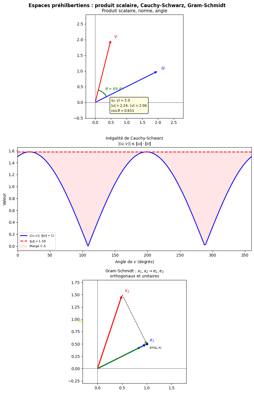
Norme et inégalité de Cauchy-Schwarz

Définition 194 (Norme euclidienne)

La norme associée au produit scalaire est \(\|x\| = \sqrt{\langle x, x\rangle}\). La distance est \(d(x, y) = \|x - y\|\).

Théorème 3 (Inégalité de Cauchy-Schwarz)

\(\forall x, y \in E\),

\[|\langle x, y\rangle| \leq \|x\| \cdot \|y\|\]

avec égalité si et seulement si \(x\) et \(y\) sont colinéaires.

Proof. Si \(y = 0\), les deux membres sont nuls. Supposons \(y \neq 0\). Pour tout \(t \in \mathbb{R}\),

\[f(t) = \|x + ty\|^2 = \|y\|^2 t^2 + 2\langle x, y\rangle t + \|x\|^2 \geq 0\]

Ce trinôme (en \(t\)) est \(\geq 0\) donc son discriminant est \(\leq 0\) : \(4\langle x, y\rangle^2 - 4\|x\|^2\|y\|^2 \leq 0\).

Égalité : \(f\) s’annule en \(t_0 = -\langle x,y\rangle/\|y\|^2\), i.e. \(x = -t_0 y\).

Proposition 278 (Propriétés de la norme)

\(\|\cdot\|\) est une norme : \(\|x\| \geq 0\), \(\|x\| = 0 \Leftrightarrow x = 0\), \(\|\lambda x\| = |\lambda|\|x\|\), \(\|x+y\| \leq \|x\|+\|y\|\).

Proof. Inégalité triangulaire : \(\|x+y\|^2 = \|x\|^2 + 2\langle x,y\rangle + \|y\|^2 \leq \|x\|^2 + 2\|x\|\|y\| + \|y\|^2 = (\|x\|+\|y\|)^2\).

Proposition 279 (Identités fondamentales)

Parallélogramme : \(\|x+y\|^2 + \|x-y\|^2 = 2(\|x\|^2 + \|y\|^2)\)

Polarisation : \(\langle x, y\rangle = \frac{1}{4}(\|x+y\|^2 - \|x-y\|^2)\)

Ces identités caractérisent les normes provenant d’un produit scalaire.

Proof. \(\|x \pm y\|^2 = \|x\|^2 \pm 2\langle x,y\rangle + \|y\|^2\). En additionnant ou soustrayant.

Orthogonalité

Définition 195 (Orthogonalité)

\(x \perp y\) si \(\langle x, y\rangle = 0\). Une famille est orthogonale si \(\langle e_i, e_j\rangle = 0\) pour \(i \neq j\), orthonormale (ONF) si de plus \(\|e_i\| = 1\).

Théorème 4 (Pythagore généralisé)

Si \((x_1, \ldots, x_k)\) est orthogonale : \(\left\|\sum_{i=1}^k x_i\right\|^2 = \sum_{i=1}^k \|x_i\|^2\).

Proposition 280 (ONF libre)

Toute famille orthogonale de vecteurs non nuls est libre.

Proof. Si \(\sum \lambda_i e_i = 0\), alors \(0 = \langle \sum_i \lambda_i e_i, e_j\rangle = \lambda_j \|e_j\|^2\), donc \(\lambda_j = 0\).

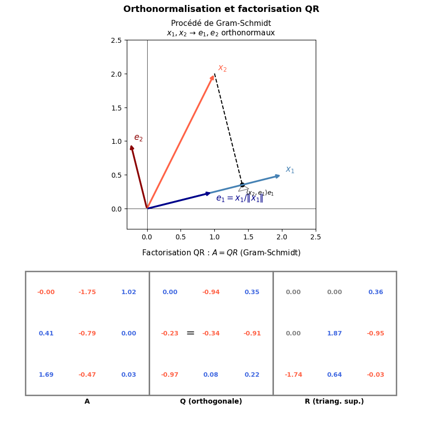
Procédé de Gram-Schmidt

Théorème 5 (Gram-Schmidt)

Soit \((x_1, \ldots, x_k)\) une famille libre. Il existe une unique ONF \((e_1, \ldots, e_k)\) telle que \(\operatorname{Vect}(e_1, \ldots, e_j) = \operatorname{Vect}(x_1, \ldots, x_j)\) et \(\langle x_j, e_j\rangle > 0\) pour tout \(j\).

Proof. Algorithme. \(e_1 = x_1/\|x_1\|\). Pour \(j \geq 2\) :

\[\tilde{e}_j = x_j - \sum_{i=1}^{j-1} \langle x_j, e_i\rangle e_i, \qquad e_j = \frac{\tilde{e}_j}{\|\tilde{e}_j\|}\]

\(\tilde{e}_j \neq 0\) car \(x_j \notin \operatorname{Vect}(x_1, \ldots, x_{j-1}) = \operatorname{Vect}(e_1, \ldots, e_{j-1})\). \(\langle \tilde{e}_j, e_i\rangle = \langle x_j, e_i\rangle - \langle x_j, e_i\rangle = 0\) pour \(i < j\).

Unicité : \(e_1\) est l’unique vecteur unitaire de \(\operatorname{Vect}(x_1)\) avec \(\langle x_1, e_1\rangle > 0\). Par récurrence.

Remarque 105

Corollaire : Tout espace euclidien admet une base orthonormale (BON).

Application : Factorisation QR d’une matrice \(A = QR\) avec \(Q\) orthogonale et \(R\) triangulaire supérieure, fondement de nombreux algorithmes numériques.

Show code cell source

Hide code cell source

import numpy as np
import matplotlib.pyplot as plt

fig, axes = plt.subplots(2, 1, figsize=(9, 9))

# --- Gram-Schmidt étape par étape (en R^3, projeté en 2D) ---
ax = axes[0]
np.random.seed(42)

# Vecteurs initiaux
x1 = np.array([2.0, 0.5])
x2 = np.array([1.0, 2.0])

# Gram-Schmidt
e1 = x1 / np.linalg.norm(x1)
proj = np.dot(x2, e1)*e1
e2_tilde = x2 - proj
e2 = e2_tilde / np.linalg.norm(e2_tilde)

# Affichage
def arrow(ax, v, c, lbl, offset=(0.05, 0.05)):
    ax.annotate('', xy=v, xytext=(0,0), arrowprops=dict(arrowstyle='->', color=c, lw=2.5))
    ax.text(v[0]+offset[0], v[1]+offset[1], lbl, fontsize=12, color=c)

arrow(ax, x1, 'steelblue', '$x_1$')
arrow(ax, x2, 'tomato', '$x_2$')
arrow(ax, e1, 'darkblue', '$e_1 = x_1/\\|x_1\\|$', (0.05, -0.12))
arrow(ax, e2, 'darkred', '$e_2$', (0.05, 0.05))

# Composante projetée
ax.plot([x2[0], proj[0]], [x2[1], proj[1]], 'k--', lw=1.5)
ax.plot(*proj, 'ko', markersize=6)
ax.annotate('$\\langle x_2, e_1\\rangle e_1$', proj, xytext=(proj[0]+0.05, proj[1]-0.15), fontsize=9)

# Angle droit
sq = 0.08
ax.add_patch(plt.Polygon([[proj[0], proj[1]],
                           [proj[0]+sq*e1[0]-sq*e2[0], proj[1]+sq*e1[1]-sq*e2[1]],
                           [proj[0]-sq*e2[0], proj[1]-sq*e2[1]],
                           [proj[0]-sq*e1[0]-sq*e2[0], proj[1]-sq*e1[1]-sq*e2[1]]],
                          fill=False, edgecolor='gray', lw=1))

ax.set_xlim(-0.3, 2.5); ax.set_ylim(-0.3, 2.5)
ax.set_aspect('equal')
ax.axhline(0, color='k', lw=0.5); ax.axvline(0, color='k', lw=0.5)
ax.set_title('Procédé de Gram-Schmidt\n$x_1, x_2$ → $e_1, e_2$ orthonormaux', fontsize=11)

# --- Factorisation QR d'une matrice 3x3 ---
ax = axes[1]
np.random.seed(7)
A = np.random.randn(3, 3)
Q, R = np.linalg.qr(A)

im = ax.imshow(np.zeros((3, 6)), cmap='Blues', vmin=-2, vmax=2, alpha=0)

# Afficher A, Q, R côte à côte
for j, (M, title, x_off) in enumerate([(A, 'A', 0), (Q, 'Q (orthogonale)', 3)]):
    for i in range(3):
        for k in range(3):
            color = 'royalblue' if M[i,k] > 0 else 'tomato'
            ax.text(x_off + k, i, f'{M[i,k]:.2f}', ha='center', va='center',
                    fontsize=9, color=color, fontweight='bold')
    ax.text(x_off + 1, -0.7, title, ha='center', fontsize=10, fontweight='bold')
    # Rectangle
    rect = plt.Rectangle((x_off - 0.5, -0.5), 3, 3, fill=False, edgecolor='gray', lw=2)
    ax.add_patch(rect)

ax.text(3.5 + 0, 1, '=', fontsize=16, ha='center', va='center')

# Afficher R (triangulaire supérieure)
for i in range(3):
    for k in range(3):
        val = R[i,k] if k >= i else 0
        color = 'royalblue' if val > 0 else ('gray' if val == 0 else 'tomato')
        ax.text(6 + k, i, f'{val:.2f}', ha='center', va='center',
                fontsize=9, color=color, fontweight='bold')
ax.text(7, -0.7, 'R (triang. sup.)', ha='center', fontsize=10, fontweight='bold')
rect = plt.Rectangle((5.5, -0.5), 3, 3, fill=False, edgecolor='gray', lw=2)
ax.add_patch(rect)

ax.set_xlim(-1, 9.5); ax.set_ylim(-1.2, 2.8)
ax.axis('off')
ax.set_title('Factorisation QR : $A = QR$ (Gram-Schmidt)', fontsize=11)

plt.suptitle('Orthonormalisation et factorisation QR', fontsize=13, fontweight='bold')
plt.tight_layout()
plt.show()

Projection orthogonale

Théorème 6 (Projection orthogonale)

Soit \(E\) euclidien et \(F\) un sous-espace vectoriel. Alors \(E = F \oplus F^\perp\). Pour tout \(x \in E\), il existe un unique \(p_F(x) \in F\) tel que \(x - p_F(x) \in F^\perp\), donné par

\[p_F(x) = \sum_{i=1}^k \langle x, e_i\rangle e_i\]

où \((e_1, \ldots, e_k)\) est une BON de \(F\). De plus, \(p_F(x)\) est le point de \(F\) le plus proche de \(x\) :

\[\|x - p_F(x)\| = \min_{y \in F} \|x - y\| = d(x, F)\]

Proof. Le produit scalaire restreint à \(F\) est défini positif, donc non dégénéré : \(F \cap F^\perp = \{0\}\) et \(\dim F + \dim F^\perp = n\) (chapitre précédent). Donc \(E = F \oplus F^\perp\).

\(p_F(x) = \sum \langle x, e_i\rangle e_i \in F\) et \(\langle x - p_F(x), e_j\rangle = \langle x, e_j\rangle - \langle x, e_j\rangle = 0\), donc \(x - p_F(x) \in F^\perp\).

Distance minimale : \(\|x-y\|^2 = \|x-p_F(x)\|^2 + \|p_F(x)-y\|^2 \geq \|x-p_F(x)\|^2\) (Pythagore, car \(x-p_F(x) \perp p_F(x)-y\)).

Proposition 281 (Inégalité de Bessel)

Soit \((e_1, \ldots, e_k)\) une ONF (pas nécessairement une base). Pour tout \(x \in E\) :

\[\sum_{i=1}^k \langle x, e_i\rangle^2 \leq \|x\|^2\]

avec égalité si et seulement si \(x \in \operatorname{Vect}(e_1, \ldots, e_k)\).

Proof. \(\|x\|^2 = \|p_F(x)\|^2 + \|x - p_F(x)\|^2 = \sum_i \langle x, e_i\rangle^2 + \|x - p_F(x)\|^2\).

Remarque 106

Application — Moindres carrés : Étant donné \(b \in \mathbb{R}^m\) et \(A \in \mathcal{M}_{m,n}(\mathbb{R})\), la solution de moindres carrés minimise \(\|Ax - b\|^2\). C’est \(x^* = (A^TA)^{-1}A^Tb\) si \(A\) est de rang plein, car \(Ax^* = p_{\operatorname{Im}A}(b)\).

Matrices orthogonales

Définition 196 (Groupe orthogonal)

\(M \in \mathcal{M}_n(\mathbb{R})\) est orthogonale si \(M^T M = I_n\) (équivalent : \(M^T = M^{-1}\), ou colonnes ONF, ou \(\|Mx\| = \|x\|\) pour tout \(x\)).

\(O_n(\mathbb{R}) = \{M : M^TM = I_n\}\) (groupe orthogonal), \(SO_n(\mathbb{R}) = \{M \in O_n : \det M = 1\}\) (groupe spécial orthogonal).

Proof. \(\det M = \pm 1\) \(1 = \det(I) = \det(M^TM) = \det(M)^2\).

Exemple 99

\(SO_2(\mathbb{R})\) : rotations \(R_\theta = \begin{pmatrix}\cos\theta & -\sin\theta \\ \sin\theta & \cos\theta\end{pmatrix}\).

\(O_2 \setminus SO_2\) : réflexions \(S_\theta = \begin{pmatrix}\cos\theta & \sin\theta \\ \sin\theta & -\cos\theta\end{pmatrix}\).

\(SO_3(\mathbb{R})\) : rotations de l’espace (3 paramètres, angles d’Euler).

Adjoint et endomorphismes symétriques

Définition 197 (Adjoint)

Soit \(E\) euclidien et \(u \in \mathcal{L}(E)\). L”adjoint \(u^*\) est l’unique endomorphisme vérifiant

\[\forall x, y \in E, \quad \langle u(x), y\rangle = \langle x, u^*(y)\rangle\]

Dans une BON, \(\operatorname{Mat}(u^*) = \operatorname{Mat}(u)^T\).

Proof. Existence : pour tout \(y\), \(x \mapsto \langle u(x), y\rangle\) est linéaire. Par représentation de Riesz (en dimension finie : l’application \(x \mapsto \langle x, z\rangle\) est bijective de \(E\) sur \(E^*\)), il existe un unique \(u^*(y)\) tel que \(\langle u(x), y\rangle = \langle x, u^*(y)\rangle\). La linéarité de \(y \mapsto u^*(y)\) est immédiate.

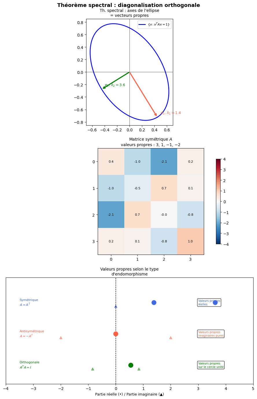
Définition 198 (Types d’endomorphismes)

• Symétrique (autoadjoint) : \(u^* = u\) (matrice symétrique dans une BON)

• Antisymétrique : \(u^* = -u\) (matrice antisymétrique)

• Orthogonal : \(u^* u = \operatorname{Id}\) (matrice orthogonale dans une BON)

• Normal (cas complexe) : \(u^* u = u u^*\)

Théorème spectral

Théorème 7 (Théorème spectral (cas réel))

Soit \(u\) un endomorphisme symétrique d’un espace euclidien \(E\). Alors :

1. Toutes les valeurs propres de \(u\) sont réelles

2. Les sous-espaces propres sont orthogonaux deux à deux

3. Il existe une BON de vecteurs propres de \(u\)

Autrement dit : toute matrice symétrique réelle \(A\) est orthogonalement diagonalisable : \(\exists P \in O_n(\mathbb{R})\) telle que \(P^T A P = D\) diagonale.

Proof. 1. Valeurs propres réelles. Soit \(\lambda\) valeur propre (complexe a priori) et \(v \neq 0\) vecteur propre, avec produit hermitien \(\langle \cdot, \cdot\rangle_{\mathbb{C}}\) sur \(\mathbb{C}^n\). \(\lambda \langle v, v\rangle_\mathbb{C} = \langle \lambda v, v\rangle_\mathbb{C} = \langle Av, v\rangle_\mathbb{C} = \langle v, A^Tv\rangle_\mathbb{C} = \langle v, Av\rangle_\mathbb{C} = \bar\lambda \langle v,v\rangle_\mathbb{C}\). Comme \(\langle v,v\rangle_\mathbb{C} > 0\) : \(\lambda = \bar\lambda \in \mathbb{R}\).

2. Sous-espaces propres orthogonaux. Si \(u(x) = \lambda x\), \(u(y) = \mu y\) avec \(\lambda \neq \mu\) : \(\lambda\langle x,y\rangle = \langle u(x),y\rangle = \langle x, u(y)\rangle = \mu\langle x,y\rangle\) Donc \((\lambda - \mu)\langle x,y\rangle = 0\), d’où \(\langle x,y\rangle = 0\).

3. BON de vecteurs propres. Par récurrence sur \(n\). Le polynôme caractéristique a ses racines réelles (par 1), donc \(u\) admet une valeur propre \(\lambda\) et un vecteur propre unitaire \(e_1\). L’orthogonal \(F = \{e_1\}^\perp\) est stable par \(u\) (car \(u\) symétrique : \(\langle u(x), e_1\rangle = \langle x, u(e_1)\rangle = \lambda\langle x, e_1\rangle = 0\)). On applique l’hypothèse de récurrence à \(u|_F\).

Remarque 107

Généralisation (cas complexe) : Tout endomorphisme normal (\(u^*u = uu^*\)) d’un espace hermitien est unitairement diagonalisable. En particulier :

• Autoadjoint (\(u^* = u\)) : valeurs propres réelles

• Unitaire (\(u^*u = I\)) : valeurs propres de module 1

• Normal : diagonalisable en BON (et toute diagonalisable dans une BON est normale)

Show code cell source

Hide code cell source

import numpy as np
import matplotlib.pyplot as plt
from matplotlib.patches import Ellipse
import seaborn as sns

fig, axes = plt.subplots(3, 1, figsize=(9, 14))

# --- Théorème spectral : ellipse = vecteurs propres ---
ax = axes[0]
A = np.array([[3., 1.], [1., 2.]])
vals, vecs = np.linalg.eigh(A)

# Unité ellipse {x : x^T A x = 1}  → demi-axes 1/sqrt(lambda_i) dans direction propre
theta = np.linspace(0, 2*np.pi, 300)
# Paramétrique : x = sum_i (1/sqrt(lambda_i)) * cos(angle_i) * e_i
# En fait x = P * diag(1/sqrt(vals)) * [cos(t), sin(t)]^T
P = vecs  # colonnes = vecteurs propres
pt = P @ np.diag(1/np.sqrt(vals)) @ np.array([np.cos(theta), np.sin(theta)])

ax.plot(pt[0], pt[1], 'b-', lw=2, label='$\\{x : x^TAx = 1\\}$')

for i, (v, lam) in enumerate(zip(vecs.T, vals)):
    scale = 1/np.sqrt(lam)
    ax.annotate('', xy=scale*v, xytext=(0,0),
                arrowprops=dict(arrowstyle='->', color=['tomato','green'][i], lw=2.5))
    ax.text(scale*v[0]+0.05, scale*v[1]+0.05, f'$e_{i+1}$, $\\lambda_{i+1}={lam:.1f}$',
            fontsize=9, color=['tomato','green'][i])

ax.set_aspect('equal')
ax.axhline(0, color='k', lw=0.5); ax.axvline(0, color='k', lw=0.5)
ax.set_title('Th. spectral : axes de l\'ellipse\n= vecteurs propres', fontsize=10)
ax.legend(fontsize=8)

# --- Diagonalisation orthogonale ---
ax = axes[1]
n = 4
np.random.seed(42)
Q_rand = np.linalg.qr(np.random.randn(n, n))[0]
D = np.diag([3., 1., -1., -2.])
A4 = Q_rand @ D @ Q_rand.T

im = ax.imshow(A4, cmap='RdBu_r', vmin=-4, vmax=4)
for i in range(n):
    for j in range(n):
        ax.text(j, i, f'{A4[i,j]:.1f}', ha='center', va='center', fontsize=8)
plt.colorbar(im, ax=ax, shrink=0.8)
ax.set_title(f'Matrice symétrique $A$\nvaleurs propres : 3, 1, −1, −2', fontsize=10)
ax.set_xticks(range(n)); ax.set_yticks(range(n))

# --- Valeurs propres sur la droite réelle ---
ax = axes[2]
matrices_names = ['Symétrique\n$A=A^T$', 'Antisymétrique\n$A=-A^T$', 'Orthogonale\n$A^TA=I$']
colors_m = ['royalblue', 'tomato', 'green']
examples = [
    np.array([[2,1],[1,3]]),
    np.array([[0,2],[-2,0]]),
    np.array([[np.cos(1),-np.sin(1)],[np.sin(1),np.cos(1)]])
]
descriptions = [
    'Valeurs propres\nréelles',
    'Valeurs propres\nimaginaires pures',
    'Valeurs propres\nsur le cercle unité'
]

y_pos = [0.75, 0.5, 0.25]
for (M, name, c, desc, y) in zip(examples, matrices_names, colors_m, descriptions, y_pos):
    eigs = np.linalg.eigvals(M)
    ax.scatter(eigs.real, [y]*len(eigs), color=c, s=120, zorder=5)
    ax.scatter(eigs.imag, [y-0.03]*len(eigs), color=c, s=40, marker='^', alpha=0.5)
    ax.text(-3.5, y, name, fontsize=8, va='center', color=c)
    ax.text(3, y, desc, fontsize=7, va='center', color=c,
            bbox=dict(boxstyle='round', facecolor='white', alpha=0.8))

ax.axvline(0, color='k', lw=1, linestyle='--')
ax.set_xlim(-4, 5); ax.set_ylim(0.1, 0.95)
ax.set_xlabel('Partie réelle (•) / Partie imaginaire (▲)', fontsize=9)
ax.set_title('Valeurs propres selon le type\nd\'endomorphisme', fontsize=10)
ax.set_yticks([])

plt.suptitle('Théorème spectral : diagonalisation orthogonale', fontsize=13, fontweight='bold')
plt.tight_layout()
plt.show()

Résumé

Concept	Résultat clé
Produit scalaire	Forme bilinéaire symétrique définie positive
Cauchy-Schwarz	\(|\langle x,y\rangle| \leq |x|\cdot|y|\), égalité ssi colinéaires
Gram-Schmidt	Famille libre → BON, même espace engendré
Projection	\(p_F(x) = \sum\langle x,e_i\rangle e_i\), minimise \(d(x,F)\)
Bessel	\(\sum\langle x,e_i\rangle^2 \leq |x|^2\)
Adjoint	\(\langle u(x),y\rangle = \langle x, u^*(y)\rangle\) ; matrice : transposée (BON)
Théorème spectral	\(u\) symétrique \(\Rightarrow\) BON de vecteurs propres, valeurs propres réelles
Groupe \(O_n\)	Matrices orthogonales, \(\det = \pm 1\), \(SO_n\) = rotations