Équations différentielles linéaires

Contenu

Équations différentielles linéaires#

Les équations différentielles sont le langage dans lequel les lois de la nature sont écrites.

— Isaac Newton

Introduction et structure générale#

Définition 129 (EDL d’ordre \(n\))

Une équation différentielle linéaire (EDL) d’ordre \(n\) est

\[a_n(t)\,y^{(n)} + a_{n-1}(t)\,y^{(n-1)} + \cdots + a_1(t)\,y' + a_0(t)\,y = b(t),\]

avec \(a_0,\ldots,a_n, b \in \mathcal{C}^0(I,\mathbb{K})\) et \(a_n \neq 0\) sur \(I\).

Proposition 204 (Structure des solutions)

Soit \(L : y \mapsto a_n y^{(n)} + \cdots + a_0 y\) l’opérateur différentiel (linéaire).

L’ensemble \(\mathcal{S}_H = \ker L\) des solutions de l”équation homogène \(Ly = 0\) est un sous-espace vectoriel de \(\mathcal{C}^n(I)\) de dimension \(n\).
L’ensemble \(\mathcal{S}\) des solutions de \(Ly = b\) est un sous-espace affine : \(\mathcal{S} = y_0 + \mathcal{S}_H\) pour toute solution particulière \(y_0\).

Proof. \(L\) est linéaire car la dérivation l’est. Donc \(\mathcal{S}_H = \ker L\) est un sev.

Si \(Ly = Lz = b\), alors \(L(y-z) = 0\), donc \(y - z \in \mathcal{S}_H\), d’où \(y \in z + \mathcal{S}_H\).

\(\dim \mathcal{S}_H = n\) : c’est la conséquence du théorème de Cauchy-Lipschitz (une solution est déterminée par ses \(n\) conditions initiales \((y(t_0), y'(t_0), \ldots, y^{(n-1)}(t_0))\)).

Remarque 84

Stratégie. Pour résoudre \(Ly = b\) :

Résoudre l’homogène \(Ly = 0\) : trouver \(\mathcal{S}_H\) (un espace vectoriel de dimension \(n\)).
Trouver une solution particulière \(y_0\) de \(Ly = b\).
Solution générale : \(y = y_0 + c_1 y_1 + \cdots + c_n y_n\), où \((y_1,\ldots,y_n)\) est une base de \(\mathcal{S}_H\).

Équations du premier ordre#

Homogène#

Proposition 205 (EDL1 homogène)

Les solutions de \(y' + a(t)\,y = 0\) (avec \(a\) continue sur \(I\)) sont

\[y(t) = C\,e^{-A(t)}, \quad C \in \mathbb{K},\]

où \(A\) est une primitive de \(a\). L’espace \(\mathcal{S}_H\) est de dimension 1.

Proof. Posons \(z(t) = y(t)\,e^{A(t)}\). Alors \(z'(t) = (y' + ay)\,e^A = 0\), donc \(z\) est constante.

Équation complète : variation de la constante#

Proposition 206 (EDL1 complète)

Les solutions de \(y' + a(t)\,y = b(t)\) sont

\[y(t) = e^{-A(t)}\!\left(C + \int b(t)\,e^{A(t)}\,dt\right).\]

Proof. On cherche une solution particulière sous la forme \(y_0 = C(t)\,e^{-A(t)}\) (variation de la constante). Alors \(y_0' + ay_0 = C'(t)\,e^{-A(t)} = b(t)\), d’où \(C'(t) = b(t)\,e^{A(t)}\).

Théorème de Cauchy-Lipschitz (ordre 1)#

Proposition 207 (Existence et unicité)

Si \(a, b \in \mathcal{C}^0(I)\) et \((t_0, y_0) \in I \times \mathbb{K}\), le problème de Cauchy

\[\begin{split}\begin{cases} y' + a(t)\,y = b(t) \\ y(t_0) = y_0 \end{cases}\end{split}\]

admet une unique solution définie sur \(I\) tout entier.

Exemple 71

\(y' - 2ty = t\) sur \(\mathbb{R}\).

Homogène : \(y_H = Ce^{t^2}\).

Variation de la constante : \(C'(t)e^{t^2} = t\), soit \(C'(t) = te^{-t^2}\), d’où \(C(t) = -\frac12 e^{-t^2}\).

Solution particulière : \(y_0 = -\frac12\). Solution générale : \(y = Ce^{t^2} - \frac12\).

Équations du second ordre à coefficients constants#

Définition 130 (EDL2 à coefficients constants)

\[y'' + ay' + by = f(t), \quad a, b \in \mathbb{K},\ f \in \mathcal{C}^0(I).\]

Proposition 208 (Solutions de l’homogène)

L”équation caractéristique \(r^2 + ar + b = 0\) (\(\Delta = a^2 - 4b\)) donne :

Cas	Racines	Solution générale de \(y''+ay'+by=0\)
\(\Delta > 0\)	\(r_1 \neq r_2 \in \mathbb{R}\)	\(C_1 e^{r_1 t} + C_2 e^{r_2 t}\)
\(\Delta = 0\)	\(r = -a/2\) (double)	\((C_1 + C_2 t)\,e^{rt}\)
\(\Delta < 0\)	\(r = \alpha \pm i\beta\)	\(e^{\alpha t}(C_1\cos\beta t + C_2\sin\beta t)\)

\(\mathcal{S}_H\) est de dimension 2 dans chaque cas.

Proof. On cherche \(y = e^{rt}\) : \((r^2 + ar + b)e^{rt} = 0 \Leftrightarrow r^2 + ar + b = 0\).

Racine double. \(e^{rt}\) est solution. Pour \(te^{rt}\) : \((te^{rt})'' + a(te^{rt})' + bte^{rt} = t(r^2+ar+b)e^{rt} + (2r+a)e^{rt} = 0\) car \(r^2+ar+b = 0\) et \(2r + a = 0\) (racine double). ✓

Racines complexes. \(e^{(\alpha+i\beta)t} = e^{\alpha t}(\cos\beta t + i\sin\beta t)\) est solution complexe. Les parties réelle et imaginaire sont deux solutions réelles indépendantes.

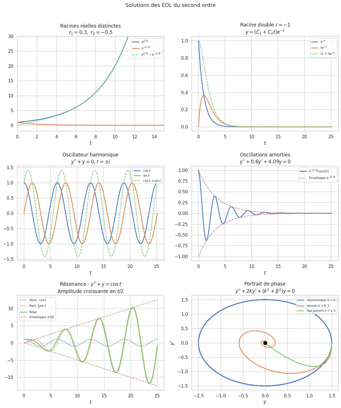
Exemple 72

\(y'' - 3y' + 2y = 0\) : \(r^2 - 3r + 2 = (r-1)(r-2)\). \(y = C_1 e^t + C_2 e^{2t}\).
\(y'' - 2y' + y = 0\) : \(r = 1\) double. \(y = (C_1 + C_2 t)e^t\).
\(y'' + y = 0\) (oscillateur harmonique) : \(r = \pm i\). \(y = C_1\cos t + C_2\sin t\).
\(y'' + 2y' + 5y = 0\) : \(r = -1 \pm 2i\). \(y = e^{-t}(C_1\cos 2t + C_2\sin 2t)\).

Solutions particulières : second membre exponentiel-polynomial#

Proposition 209 (Méthode d’identification)

Pour \(y'' + ay' + by = P(t)e^{\alpha t}\) (\(P\) polynôme de degré \(d\)) :

\(\alpha\) non racine de l’éq. car. : \(y_0 = Q(t)e^{\alpha t}\) avec \(\deg Q = d\)
\(\alpha\) racine simple : \(y_0 = tQ(t)e^{\alpha t}\)
\(\alpha\) racine double : \(y_0 = t^2 Q(t)e^{\alpha t}\)

Pour \(P(t)e^{\alpha t}\cos(\beta t)\) ou \(P(t)e^{\alpha t}\sin(\beta t)\) : on traite \(P(t)e^{(\alpha+i\beta)t}\) et on prend Re ou Im.

Exemple 73

Résonance. \(y'' + y = \cos t\) : \(\alpha = i\) est racine simple de \(r^2 + 1 = 0\).

On cherche \(\mathrm{Re}(te^{it} \cdot A)\). \((te^{it})'' + te^{it} = 2ie^{it} = 1 \cdot e^{it}\), donc \(2iA = 1\), \(A = \frac{1}{2i} = -\frac{i}{2}\).

\(y_0 = \mathrm{Re}\left(-\frac{it}{2}e^{it}\right) = \frac{t}{2}\sin t\) (résonance : amplitude croissante).

Solution générale : \(y = C_1\cos t + C_2\sin t + \frac{t}{2}\sin t\).

Show code cell source

Hide code cell source

import numpy as np
import matplotlib.pyplot as plt
import seaborn as sns
from scipy.integrate import solve_ivp

sns.set_theme(style="whitegrid", palette="muted", font_scale=1.0)

fig, axes = plt.subplots(3, 2, figsize=(12, 14))

t = np.linspace(0, 8*np.pi, 1000)

# 1. Racines réelles distinctes
y1 = np.exp(0.3*t); y2 = np.exp(-0.5*t)
axes[0,0].plot(t, y1, 'C0-', lw=2, label='$e^{0.3t}$')
axes[0,0].plot(t, y2, 'C1-', lw=2, label='$e^{-0.5t}$')
axes[0,0].plot(t, y1 - y2, 'C2--', lw=1.5, label='$e^{0.3t} - e^{-0.5t}$')
axes[0,0].set(xlim=(0, 15), ylim=(-2, 30), xlabel='$t$',
              title='Racines réelles distinctes\n$r_1=0.3,\\ r_2=-0.5$')
axes[0,0].legend(fontsize=8)

# 2. Racine double
y_double = (1 + t) * np.exp(-t)
y_base = np.exp(-t)
axes[0,1].plot(t, y_base, 'C0-', lw=2, label='$e^{-t}$')
axes[0,1].plot(t, t*np.exp(-t), 'C1-', lw=2, label='$te^{-t}$')
axes[0,1].plot(t, y_double, 'C2--', lw=1.5, label='$(1+t)e^{-t}$')
axes[0,1].set(xlabel='$t$', title='Racine double $r=-1$\n$y=(C_1+C_2t)e^{-t}$')
axes[0,1].legend(fontsize=8)

# 3. Racines complexes : oscillations
# Harmonique
axes[1,0].plot(t, np.cos(t), 'C0-', lw=2, label='$\\cos t$')
axes[1,0].plot(t, np.sin(t), 'C1-', lw=2, label='$\\sin t$')
axes[1,0].plot(t, np.cos(t) + np.sin(t), 'C2--', lw=1.5, label='$\\cos t + \\sin t$')
axes[1,0].set(xlabel='$t$', title='Oscillateur harmonique\n$y\'\'+y=0$, $r=\\pm i$')
axes[1,0].legend(fontsize=8)

# 4. Oscillations amorties
alpha, beta = -0.3, 2.0
y_amort = np.exp(alpha*t) * np.cos(beta*t)
env = np.exp(alpha*t)
axes[1,1].plot(t, y_amort, 'C0-', lw=2, label='$e^{-0.3t}\\cos(2t)$')
axes[1,1].plot(t, env, 'C3--', lw=1.5, alpha=0.8, label='Enveloppe $e^{-0.3t}$')
axes[1,1].plot(t, -env, 'C3--', lw=1.5, alpha=0.8)
axes[1,1].set(xlabel='$t$', title='Oscillations amorties\n$y\'\'+0.6y\'+4.09y=0$')
axes[1,1].legend(fontsize=8)

# 5. Résonance : y'' + y = cos(t)
t_res = np.linspace(0, 25, 1000)
y_hom = np.cos(t_res)           # solution homogène
y_part = t_res/2 * np.sin(t_res) # solution particulière (résonance)
y_tot = y_hom + y_part
axes[2,0].plot(t_res, y_hom, 'C0-', lw=1.5, alpha=0.6, label='Hom. $\\cos t$')
axes[2,0].plot(t_res, y_part, 'C1-', lw=1.5, alpha=0.6, label='Part. $\\frac{t}{2}\\sin t$')
axes[2,0].plot(t_res, y_tot, 'C2-', lw=2, label='Total')
axes[2,0].plot(t_res, t_res/2, 'C3--', lw=1.5, alpha=0.7, label='Enveloppe $\\pm t/2$')
axes[2,0].plot(t_res, -t_res/2, 'C3--', lw=1.5, alpha=0.7)
axes[2,0].set(xlabel='$t$', title='Résonance : $y\'\'+y = \\cos t$\nAmplitude croissante en $t/2$')
axes[2,0].legend(fontsize=8)

# 6. Portrait de phase (EDL2 homogène)
# Oscillateur amorti : y'' + 2ky' + w^2*y = 0
ax6 = axes[2,1]
ax6.set(xlabel='$y$', ylabel='$y\'$', title='Portrait de phase\n$y\'\'+2ky\'+(k^2+\\beta^2)y=0$')
for k, beta_val, col, lbl in [(0, 1, 'C0', 'Harmonique $k=0$'),
                                (0.3, 1, 'C1', 'Amorti $k=0.3$'),
                                (1.5, 0, 'C2', 'Sur-amorti $k=1.5$')]:
    def edl(t, Y, k=k, beta_val=beta_val):
        y, yp = Y
        return [yp, -(2*k)*yp - (k**2+beta_val**2)*y]
    y0_vec = [1.5, 0]
    sol = solve_ivp(edl, [0, 20], y0_vec, dense_output=True, max_step=0.05)
    ax6.plot(sol.y[0], sol.y[1], col+'-', lw=2, label=lbl)
ax6.scatter([0],[0], s=80, color='black', zorder=5)
ax6.legend(fontsize=8)

plt.suptitle('Solutions des EDL du second ordre', fontsize=13, y=1.01)
plt.tight_layout()
plt.show()

_images/e8d1fa1d9e7f6f4c456586c824205f804d4b6ecbdf61465e48c3b67137b98a14.png

Wronskien et indépendance des solutions#

Définition 131 (Wronskien)

Le wronskien de \((y_1, \ldots, y_n)\) est

\[\begin{split}W(t) = \det\begin{pmatrix} y_1 & \cdots & y_n \\ y_1' & \cdots & y_n' \\ \vdots && \vdots \\ y_1^{(n-1)} & \cdots & y_n^{(n-1)} \end{pmatrix}.\end{split}\]

Proposition 210 (Critère d’indépendance)

\((y_1, \ldots, y_n)\) solutions de \(Ly = 0\) sont linéairement indépendantes (base de \(\mathcal{S}_H\)) \(\iff\) \(W(t_0) \neq 0\) pour un (et alors tout) \(t_0 \in I\).

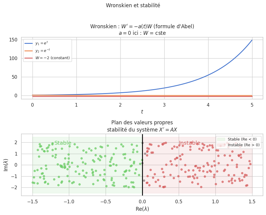
Proposition 211 (Formule d’Abel (Liouville))

Si \(y_1, y_2\) sont solutions de \(y'' + a(t)y' + b(t)y = 0\) :

\[W'(t) = -a(t)\,W(t), \qquad W(t) = W(t_0)\,e^{-\int_{t_0}^t a(s)\,ds}.\]

En particulier : \(W \equiv 0\) ou \(W\) ne s’annule jamais.

Proof. \(W = y_1 y_2' - y_2 y_1'\). \(W' = y_1 y_2'' - y_2 y_1'' = y_1(-ay_2'-by_2) - y_2(-ay_1'-by_1) = -a(y_1y_2'-y_2y_1') = -aW\).

Variation des constantes (ordre 2)#

Proposition 212 (Méthode de variation des constantes)

Soit \((y_1, y_2)\) base de \(\mathcal{S}_H\). On cherche \(y_0 = C_1(t)y_1 + C_2(t)y_2\) avec la contrainte \(C_1'y_1 + C_2'y_2 = 0\) (système de Lagrange) :

\[\begin{split}\begin{cases} C_1'y_1 + C_2'y_2 = 0 \\ C_1'y_1' + C_2'y_2' = f \end{cases}\end{split}\]

Le déterminant est \(W \neq 0\), donc :

\[C_1'(t) = -\frac{y_2(t)f(t)}{W(t)}, \qquad C_2'(t) = \frac{y_1(t)f(t)}{W(t)}.\]

Exemple 74

\(y'' + y = \frac{1}{\cos t}\) sur \(]-\pi/2, \pi/2[\).

Homogène : \(y_1 = \cos t\), \(y_2 = \sin t\), \(W = 1\).

\(C_1'(t) = -\sin t / \cos t = -\tan t\), \(C_1 = \ln|\cos t|\). \(C_2'(t) = 1\), \(C_2 = t\).

\(y_0 = \cos t \cdot \ln|\cos t| + t\sin t\).

EDL d’ordre \(n\) à coefficients constants#

Proposition 213 (Solution de l’homogène (ordre \(n\)))

Si l’équation caractéristique \(r^n + a_{n-1}r^{n-1} + \cdots + a_0 = 0\) admet les racines \(r_1,\ldots,r_p\) de multiplicités \(m_1,\ldots,m_p\) (\(\sum m_i = n\)), alors :

\[y_H(t) = \sum_{k=1}^p P_k(t)\,e^{r_k t},\]

où \(P_k\) est un polynôme de degré \(< m_k\) (à \(m_k\) constantes arbitraires).

Exemple 75

\(y^{(4)} + 2y'' + y = 0\) : \(r^4 + 2r^2 + 1 = (r^2+1)^2 = 0\), racines \(\pm i\) (mult. 2).

\[y = (C_1 + C_2 t)\cos t + (C_3 + C_4 t)\sin t.\]

Systèmes différentiels linéaires#

Définition 132 (Système différentiel linéaire)

\[X'(t) = A(t)\,X(t) + B(t), \quad X : I \to \mathbb{K}^n,\ A \in \mathcal{C}^0(I, \mathcal{M}_n).\]

Proposition 214 (Théorème de Cauchy-Lipschitz (ordre \(n\)))

Pour tout \((t_0, X_0) \in I \times \mathbb{K}^n\), le problème de Cauchy \(X' = AX + B\), \(X(t_0) = X_0\) admet une unique solution définie sur \(I\) tout entier.

Proposition 215 (Réduction par diagonalisation)

Si \(A\) est diagonalisable : \(A = PDP^{-1}\), \(D = \mathrm{diag}(\lambda_i)\). Le changement \(X = PY\) transforme \(X' = AX\) en \(Y' = DY\) (système découplé) :

\[y_i' = \lambda_i\,y_i \implies y_i(t) = C_i\,e^{\lambda_i t}.\]

D’où \(X(t) = P\,\mathrm{diag}(e^{\lambda_i t})\,\mathbf{C}\) avec \(\mathbf{C} = P^{-1}X_0\).

Proposition 216 (Solution par exponentielle de matrice)

La solution de \(X' = AX\), \(X(0) = X_0\) (avec \(A\) constante) est

\[X(t) = e^{tA}\,X_0, \quad \text{où } e^{tA} = \sum_{k=0}^{+\infty} \frac{t^k A^k}{k!}.\]

Proof. \(\Phi(t) = e^{tA}\) vérifie \(\Phi'(t) = A\Phi(t)\) (dériver terme à terme) et \(\Phi(0) = I_n\).

Show code cell source

Hide code cell source

fig, axes = plt.subplots(3, 1, figsize=(9, 11))

# 1. Système 2D : portrait de phase
from scipy.integrate import solve_ivp

A_sys = np.array([[1., 2.], [-1., 0.]])
eigs, P = np.linalg.eig(A_sys)
print(f"Valeurs propres : {eigs}")

ax = axes[0]
ax.set(xlim=(-3, 3), ylim=(-3, 3), aspect='equal',
       xlabel='$x_1$', ylabel='$x_2$',
       title=f'Portrait de phase : $X\' = AX$\n$\\lambda = {eigs[0]:.2f}, {eigs[1]:.2f}$')

# Champ de vecteurs
x1g, x2g = np.meshgrid(np.linspace(-3,3,15), np.linspace(-3,3,15))
dx1 = A_sys[0,0]*x1g + A_sys[0,1]*x2g
dx2 = A_sys[1,0]*x1g + A_sys[1,1]*x2g
norm = np.sqrt(dx1**2 + dx2**2 + 1e-10)
ax.quiver(x1g, x2g, dx1/norm, dx2/norm, alpha=0.4, color='gray', scale=30)

# Trajectoires
for x0, col in [([1,0],'C0'), ([0,1],'C1'), ([-1,0],'C2'), ([0,-1],'C3')]:
    sol = solve_ivp(lambda t, X: A_sys @ X, [0, 2], x0, dense_output=True, max_step=0.02)
    ax.plot(sol.y[0], sol.y[1], col+'-', lw=2)
    ax.scatter([x0[0]], [x0[1]], s=40, color=col, zorder=5)
# Directions propres
for i, (val, vec) in enumerate(zip(eigs, P.T)):
    t_line = np.linspace(-3, 3, 50)
    ax.plot(vec.real[0]*t_line/max(abs(vec.real)),
            vec.real[1]*t_line/max(abs(vec.real)), '--', lw=1.5, alpha=0.7, color=f'C{i}',
            label=f'$v_{i+1}$ ($\\lambda={val:.2f}$)')
ax.legend(fontsize=7, loc='upper left')

# 2. Système stable vs instable (spirales)
cases = [
    (np.array([[-0.5, 2.], [-2., -0.5]]), 'Spirale stable\n$\\mathrm{Re}(\\lambda)<0$', 'C0'),
    (np.array([[0.3, 2.], [-2., 0.3]]), 'Spirale instable\n$\\mathrm{Re}(\\lambda)>0$', 'C3'),
]
for ax_idx, (A_sp, title, col) in zip([1,2], cases):
    ax_s = axes[ax_idx]
    eigs_sp = np.linalg.eigvals(A_sp)
    x1g, x2g = np.meshgrid(np.linspace(-2,2,12), np.linspace(-2,2,12))
    dx1 = A_sp[0,0]*x1g + A_sp[0,1]*x2g
    dx2 = A_sp[1,0]*x1g + A_sp[1,1]*x2g
    norm = np.sqrt(dx1**2 + dx2**2 + 1e-10)
    ax_s.quiver(x1g, x2g, dx1/norm, dx2/norm, alpha=0.3, color='gray', scale=30)

    t_end = 10 if 'stable' in title else 3
    for x0, c in [([1.5,0],'C0'), ([0,1.5],'C1'), ([-1,0],'C2')]:
        try:
            sol = solve_ivp(lambda t, X, A=A_sp: A @ X, [0, t_end], x0,
                           dense_output=True, max_step=0.05)
            ax_s.plot(sol.y[0], sol.y[1], c+'-', lw=2)
        except: pass

    ax_s.scatter([0],[0], s=80, color='black', zorder=5)
    lam_str = f'$\\lambda = {eigs_sp[0].real:.1f} \\pm {abs(eigs_sp[0].imag):.1f}i$'
    ax_s.set(xlim=(-2.5,2.5), ylim=(-2.5,2.5), aspect='equal',
             xlabel='$x_1$', ylabel='$x_2$', title=f'{title}\n{lam_str}')

plt.suptitle('Systèmes différentiels linéaires', fontsize=12, y=1.02)
plt.tight_layout()
plt.show()

Valeurs propres : [0.5+1.32287566j 0.5-1.32287566j]

_images/0cb80388fb6c22c24b90eefd4df0a7de141c26dba582f42ea1c0e0d19f3669a4.png

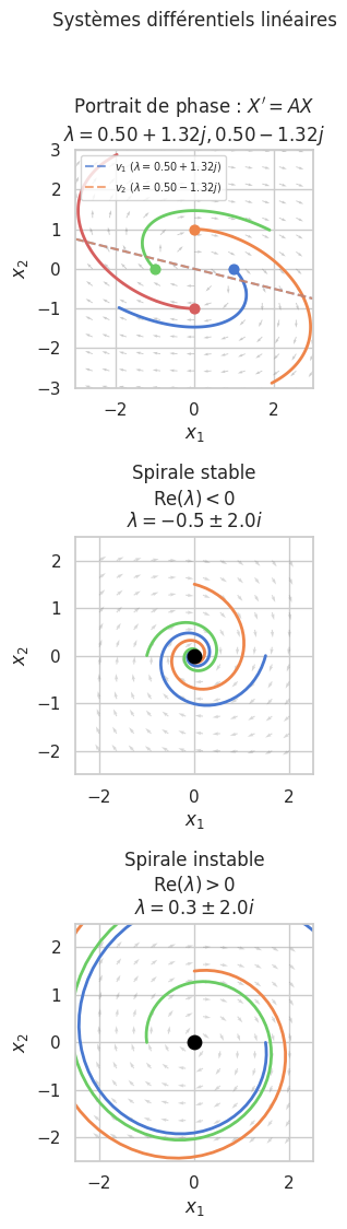
Stabilité des systèmes linéaires#

Définition 133 (Stabilité)

Le point d’équilibre \(0\) du système \(X' = AX\) est :

stable si tout \(X(t) \to 0\) quand \(t \to +\infty\)
marginalement stable si les trajectoires restent bornées
instable sinon

Proposition 217 (Critère de stabilité)

Spectre de \(A\)	Comportement
Toutes les VP : \(\mathrm{Re}(\lambda) < 0\)	Stable (spirale/nœud stable)
\(\mathrm{Re}(\lambda) \leq 0\), parties imaginaires pures simples	Marginal
Au moins une VP : \(\mathrm{Re}(\lambda) > 0\)	Instable

Remarque 85

Pour un système \(X' = AX\) stable, toutes les solutions \(X(t) \to 0\) exponentiellement vite, à la vitesse \(e^{\max_\lambda \mathrm{Re}(\lambda) \cdot t}\).

_images/0a65bd4653f38d09bf0020f9937d5fce64427127b84e2ac91e2c91a6d1c0dbcb.png