Déterminants

Le déterminant est le volume signé de la transformation.

— Carl Friedrich Gauss

Permutations et signature

Définition 164 (Permutation et groupe symétrique)

Une permutation de \(\{1,\ldots,n\}\) est une bijection \(\sigma : \{1,\ldots,n\} \to \{1,\ldots,n\}\).

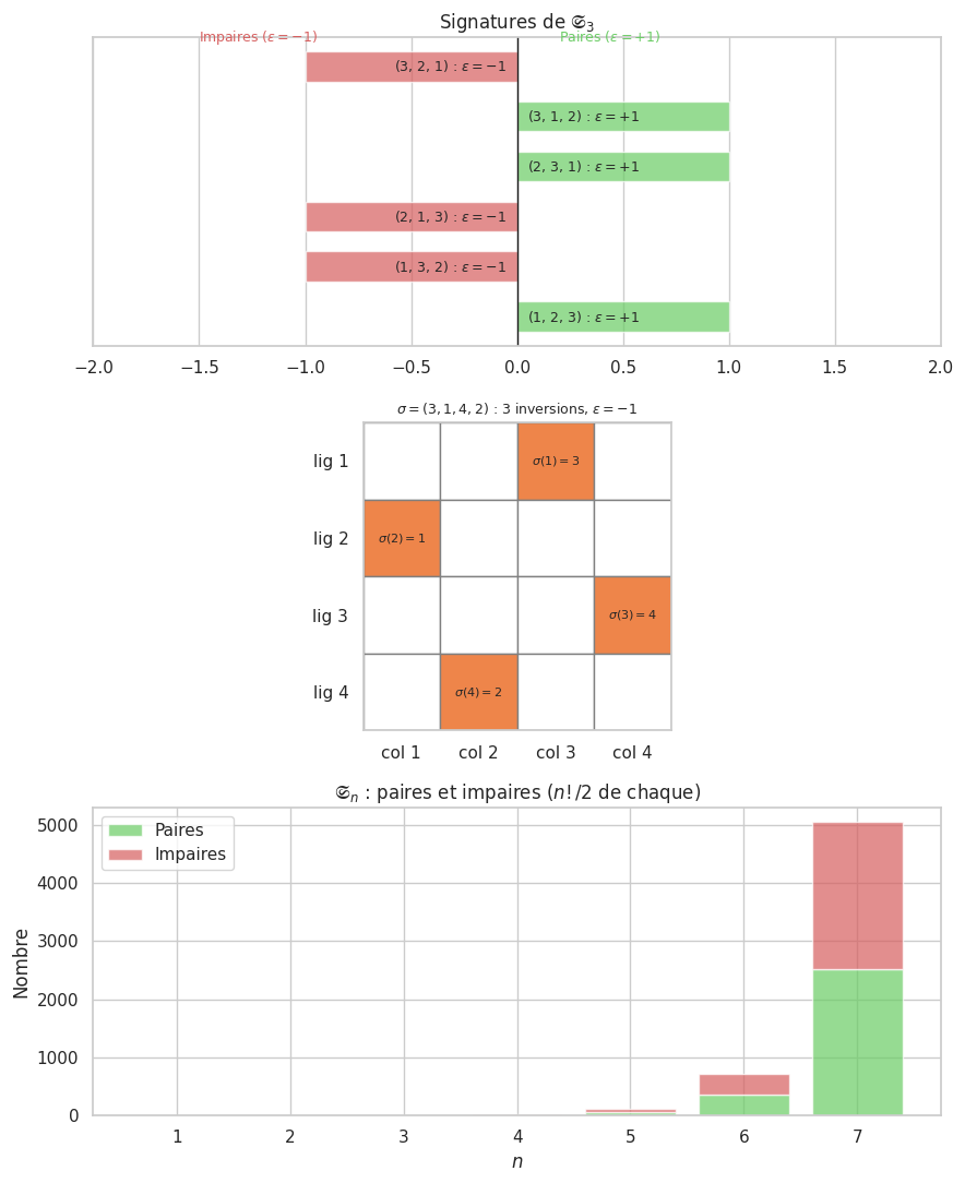
\(\mathfrak{S}_n\) est le groupe symétrique d’ordre \(n! = |\mathfrak{S}_n|\). C’est le groupe (non abélien pour \(n \geq 3\)) des permutations, de loi \(\circ\).

Définition 165 (Transposition et signature)

Une transposition \(\tau_{ij}\) échange \(i\) et \(j\) (fixe les autres).

Toute permutation est un produit de transpositions. La signature \(\varepsilon : \mathfrak{S}_n \to \{+1,-1\}\) est l’unique morphisme de groupes vérifiant \(\varepsilon(\tau) = -1\) pour toute transposition :

\[\varepsilon(\sigma) = (-1)^{\#\text{inversions}(\sigma)}, \qquad \text{inversions}(\sigma) = \{(i,j) : i < j,\ \sigma(i) > \sigma(j)\}.\]

Proposition 248 (Propriétés de la signature)

• \(\varepsilon(\sigma \circ \tau) = \varepsilon(\sigma)\,\varepsilon(\tau)\) (morphisme)

• \(\varepsilon(\sigma^{-1}) = \varepsilon(\sigma)\)

• \(\varepsilon(\text{id}) = +1\), \(\varepsilon(\tau_{ij}) = -1\)

• Un \(k\)-cycle \(\varepsilon = (-1)^{k-1}\)

Show code cell source

Hide code cell source

import numpy as np
import matplotlib.pyplot as plt
import seaborn as sns
import math
from itertools import permutations

sns.set_theme(style="whitegrid", palette="muted", font_scale=1.0)

def signature(perm):
    """Calcule la signature d'une permutation (0-indexée)."""
    n = len(perm)
    visited = [False]*n
    sign = 1
    for i in range(n):
        if not visited[i]:
            j, cycle_len = i, 0
            while not visited[j]:
                visited[j] = True
                j = perm[j]
                cycle_len += 1
            sign *= (-1)**(cycle_len - 1)
    return sign

fig, axes = plt.subplots(3, 1, figsize=(9, 11))

# S_3 : affichage de toutes les permutations avec signature
perms = list(permutations([0,1,2]))
sigs = [signature(p) for p in perms]
perm_labels = [str(tuple(i+1 for i in p)) for p in perms]
colors = ['C2' if s == 1 else 'C3' for s in sigs]

ax = axes[0]
for i, (lbl, s, c) in enumerate(zip(perm_labels, sigs, colors)):
    ax.barh(i, s, color=c, alpha=0.7, height=0.6)
    ax.text(0.05*s, i, f'{lbl} : $\\varepsilon = {s:+d}$', va='center', fontsize=9,
            ha='left' if s > 0 else 'right')
ax.axvline(0, color='k', lw=1)
ax.set(xlim=(-2, 2), title='Signatures de $\\mathfrak{S}_3$', yticks=[])
ax.text(-1.5, 5.5, 'Impaires ($\\varepsilon=-1$)', color='C3', fontsize=9)
ax.text(0.2, 5.5, 'Paires ($\\varepsilon=+1$)', color='C2', fontsize=9)

# Inversions dans une permutation
ax2 = axes[1]
sigma = (2, 0, 3, 1)  # 0-indexé : σ = (3,1,4,2) en 1-indexé
n = len(sigma)
ax2.set(xlim=(-0.5, n-0.5), ylim=(-0.5, n-0.5), aspect='equal',
        title=f'Permutation $\\sigma=(3,1,4,2)$ : inversions')
for i in range(n):
    for j in range(n):
        color = 'C1' if j == sigma[i] else 'white'
        ax2.add_patch(plt.Rectangle((j-0.5, n-1-i-0.5), 1, 1,
                                     facecolor=color, edgecolor='gray'))
        if j == sigma[i]:
            ax2.text(j, n-1-i, f'$\\sigma({i+1})={sigma[i]+1}$', ha='center',
                     va='center', fontsize=8)
# Marquer les inversions
inv_count = 0
for i in range(n):
    for j in range(i+1, n):
        if sigma[i] > sigma[j]:
            inv_count += 1
ax2.set_title(f'$\\sigma=(3,1,4,2)$ : {inv_count} inversions, $\\varepsilon = {(-1)**inv_count:+d}$',
              fontsize=9)
ax2.set_xticks(range(n)); ax2.set_xticklabels([f'col {j+1}' for j in range(n)])
ax2.set_yticks(range(n)); ax2.set_yticklabels([f'lig {n-i}' for i in range(n)])

# Nombres de permutations paires/impaires par n
ns = range(1, 8)
pairs = [len([p for p in permutations(range(k)) if signature(p)==1]) for k in ns]
impairs = [len([p for p in permutations(range(k)) if signature(p)==-1]) for k in ns]
totals = [math.factorial(k) for k in ns]

ax3 = axes[2]
ax3.bar(list(ns), pairs, label='Paires', color='C2', alpha=0.7)
ax3.bar(list(ns), impairs, bottom=pairs, label='Impaires', color='C3', alpha=0.7)
ax3.set(xlabel='$n$', ylabel='Nombre', title='$\\mathfrak{S}_n$ : paires et impaires ($n!/2$ de chaque)')
ax3.legend()

plt.tight_layout()
plt.show()

Formes multilinéaires alternées et déterminant

Définition 166 (Forme \(n\)-linéaire alternée)

\(\varphi : E^n \to \mathbb{K}\) est \(n\)-linéaire alternée si elle est linéaire en chaque variable (les autres fixées) et s’annule dès que deux arguments sont égaux.

Proposition 249 (Propriétés)

Si \(\varphi\) est \(n\)-linéaire alternée :

• Antisymétrie : l’échange de deux arguments change le signe

• Famille liée : \(\varphi(v_1,\ldots,v_n) = 0\) si \((v_i)\) est liée

• Action des permutations : \(\varphi(v_{\sigma(1)},\ldots,v_{\sigma(n)}) = \varepsilon(\sigma)\,\varphi(v_1,\ldots,v_n)\)

L’espace des formes \(n\)-linéaires alternées sur un ev de dimension \(n\) est de dimension 1.

Définition 167 (Déterminant)

Le déterminant de \(A = (a_{ij}) \in \mathcal{M}_n(\mathbb{K})\) est l’unique forme \(n\)-linéaire alternée en les colonnes valant \(1\) sur \(I_n\) :

\[\det A = \sum_{\sigma \in \mathfrak{S}_n} \varepsilon(\sigma) \prod_{i=1}^n a_{i,\sigma(i)}.\]

Exemple 87

\[\begin{split}\det\begin{pmatrix}a&b\\c&d\end{pmatrix} = ad - bc.\end{split}\]

Règle de Sarrus (dimension 3) :

\[\begin{split}\det\begin{pmatrix}a&b&c\\d&e&f\\g&h&i\end{pmatrix} = aei + bfg + cdh - ceg - bdi - afh.\end{split}\]

Propriétés fondamentales

Proposition 250 (Propriétés du déterminant)

Soit \(A, B \in \mathcal{M}_n(\mathbb{K})\).

1. \(\det(I_n) = 1\)

2. \(\det(A^T) = \det(A)\)

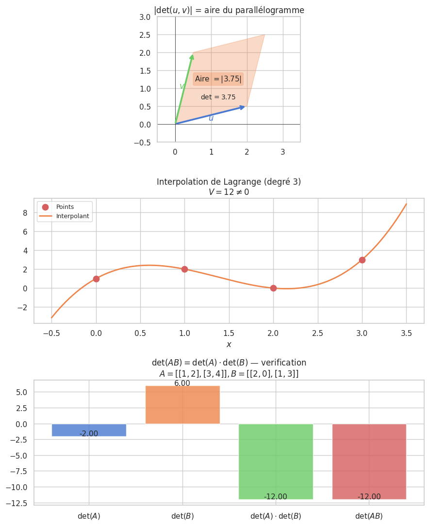
3. \(\det(AB) = \det(A)\,\det(B)\) (morphisme multiplicatif)

4. \(A \in GL_n(\mathbb{K}) \iff \det(A) \neq 0\), et \(\det(A^{-1}) = 1/\det(A)\)

5. \(\det(\lambda A) = \lambda^n \det(A)\)

6. \(\det(P^{-1}AP) = \det(A)\) (invariant par similitude)

Proof. \(\det(AB) = \det(A)\det(B)\). Si \(B\) est inversible, l’application \(A \mapsto \det(AB)\) est \(n\)-linéaire alternée en les colonnes de \(A\), valant \(\det(B)\) pour \(A = I_n\). Par unicité, \(\det(AB) = \det(B)\det(A)\). Si \(B\) n’est pas inversible, \(AB\) ne l’est pas non plus, donc \(\det(AB) = 0 = \det(A) \cdot 0\).

Proposition 251 (Effet des opérations élémentaires)

Opération	Effet sur \(\det\)
\(L_i \leftrightarrow L_j\)	Multiplie par \(-1\)
\(L_i \leftarrow \lambda L_i\)	Multiplie par \(\lambda\)
\(L_i \leftarrow L_i + \lambda L_j\)	Inchangé

Remarque 91

En pratique, on calcule \(\det(A)\) par pivot de Gauss : on met \(A\) sous forme triangulaire \(T\) en notant les opérations effectuées, puis \(\det(A) = (\pm 1)^{\text{nb échanges}} \cdot \prod_i T_{ii}\).

Calcul par développement

Définition 168 (Mineur et cofacteur)

Le mineur \(M_{ij}\) est le déterminant de la sous-matrice obtenue en supprimant la ligne \(i\) et la colonne \(j\).

Le cofacteur est \(C_{ij} = (-1)^{i+j} M_{ij}\).

Proposition 252 (Développement par rapport à une ligne/colonne)

\[\det(A) = \sum_{j=1}^n a_{ij} C_{ij} \quad \text{(ligne } i\text{)} \qquad = \sum_{i=1}^n a_{ij} C_{ij} \quad \text{(colonne } j\text{)}.\]

Exemple 88

\[\begin{split}\det\begin{pmatrix}2&1&3\\0&4&1\\1&0&2\end{pmatrix} = 2(8-0) - 0 + 1(1-12) = 16 - 11 = 5.\end{split}\]

(développement par la 1ère colonne)

Proposition 253 (Matrices triangulaires)

\[\begin{split}\det\begin{pmatrix}d_1 & * \\ & \ddots \\ 0 & d_n\end{pmatrix} = \prod_{i=1}^n d_i.\end{split}\]

Déterminant de Vandermonde

Proposition 254 (Déterminant de Vandermonde)

\[\begin{split}V(x_1,\ldots,x_n) = \det\begin{pmatrix}1&1&\cdots&1\\x_1&x_2&\cdots&x_n\\\vdots&&\ddots&\vdots\\x_1^{n-1}&x_2^{n-1}&\cdots&x_n^{n-1}\end{pmatrix} = \prod_{1\leq i < j \leq n}(x_j - x_i).\end{split}\]

Non nul \(\iff\) les \(x_i\) sont deux à deux distincts.

Proof. \(V\) est un polynôme en \(x_1,\ldots,x_n\). Si \(x_i = x_j\), deux colonnes sont égales donc \(V = 0\), i.e. \((x_j - x_i) \mid V\). Les facteurs \(\prod_{i<j}(x_j-x_i)\) (degré \(\binom{n}{2}\)) divisent \(V\) (même degré), à constante près. Le coefficient dominant est 1 (par récurrence).

Remarque 92

Application à l”interpolation de Lagrange : par \(n\) points \((x_i, y_i)\) à abscisses distinctes, il existe un unique polynôme de degré \(\leq n-1\). Le système \((x_i^j)_{ij}\) est le transposé de Vandermonde, inversible car \(V \neq 0\).

Show code cell source

Hide code cell source

fig, axes = plt.subplots(3, 1, figsize=(9, 11))

# 1. Interprétation géométrique : det = aire/volume
ax = axes[0]
ax.set(xlim=(-0.5, 3.5), ylim=(-0.5, 3), aspect='equal',
       title='$|\\det(u,v)|$ = aire du parallélogramme')
ax.axhline(0, color='k', lw=0.5); ax.axvline(0, color='k', lw=0.5)
u = np.array([2, 0.5])
v = np.array([0.5, 2])
# Parallélogramme
parallelogram = plt.Polygon([np.zeros(2), u, u+v, v], alpha=0.3, color='C1')
ax.add_patch(parallelogram)
ax.annotate('', xy=u, xytext=(0,0), arrowprops=dict(arrowstyle='->', color='C0', lw=2.5))
ax.annotate('', xy=v, xytext=(0,0), arrowprops=dict(arrowstyle='->', color='C2', lw=2.5))
ax.text(u[0]/2, u[1]/2-0.15, '$u$', fontsize=12, color='C0', ha='center')
ax.text(v[0]/2-0.15, v[1]/2, '$v$', fontsize=12, color='C2')
det_val = u[0]*v[1] - u[1]*v[0]
ax.text(1.2, 1.2, f'Aire $= |{det_val:.2f}|$', fontsize=11, ha='center',
        bbox=dict(boxstyle='round', facecolor='C1', alpha=0.3))
ax.text(1.2, 0.7, f'$\\det = {det_val:.2f}$', fontsize=10, ha='center')

# 2. Vandermonde et interpolation
ax2 = axes[1]
xs = np.array([0., 1., 2., 3.])
ys = np.array([1., 2., 0., 3.])
# Matrice de Vandermonde
Vand = np.vander(xs, increasing=True)
coeffs = np.linalg.solve(Vand, ys)
x_plot = np.linspace(-0.5, 3.5, 200)
y_plot = sum(c*x_plot**k for k,c in enumerate(coeffs))
ax2.scatter(xs, ys, s=80, color='C3', zorder=5, label='Points')
ax2.plot(x_plot, y_plot, 'C1-', lw=2, label='Interpolant')
ax2.set(xlabel='$x$', title=f'Interpolation de Lagrange (degré 3)\n$V ={np.linalg.det(Vand):.0f} \\neq 0$')
ax2.legend(fontsize=9)

# 3. det(AB) = det(A)*det(B) : visualisation
n_trials = 500
np.random.seed(0)
dets_A = np.random.randn(n_trials)
dets_B = np.random.randn(n_trials)
dets_AB = dets_A * dets_B
dets_AB_computed = np.array([
    np.linalg.det(
        np.random.randn(3,3) * abs(dets_A[i])**(1/3)
        @ np.random.randn(3,3) * abs(dets_B[i])**(1/3)
    ) for i in range(50)
])

ax3 = axes[2]
# Simple illustration numérique
A_ex = np.array([[1.,2.],[3.,4.]])
B_ex = np.array([[2.,0.],[1.,3.]])
dA, dB, dAB = np.linalg.det(A_ex), np.linalg.det(B_ex), np.linalg.det(A_ex@B_ex)
labels = ['$\\det(A)$', '$\\det(B)$', '$\\det(A)\\cdot\\det(B)$', '$\\det(AB)$']
vals = [dA, dB, dA*dB, dAB]
colors = ['C0', 'C1', 'C2', 'C3']
bars = ax3.bar(labels, vals, color=colors, alpha=0.8)
for bar, val in zip(bars, vals):
    ax3.text(bar.get_x()+bar.get_width()/2, bar.get_height()+0.05,
             f'{val:.2f}', ha='center', fontsize=11)
ax3.set_title(r'$\det(AB) = \det(A)\cdot\det(B)$ — verification' + 
        '\n$A=[[1,2],[3,4]], B=[[2,0],[1,3]]$')

plt.tight_layout()
plt.show()

Comatrice, formule de l’inverse, et formules de Cramer

Définition 169 (Comatrice)

La comatrice de \(A\) est \(\mathrm{com}(A) = (C_{ij})^T\) (transposée de la matrice des cofacteurs).

Proposition 255 (Formule de l’inverse)

\[A \cdot \mathrm{com}(A) = \det(A) \cdot I_n, \qquad \text{donc si } \det(A)\neq 0 : \quad A^{-1} = \frac{1}{\det(A)}\,\mathrm{com}(A).\]

Proof. \((A \cdot \mathrm{com}(A))_{ik} = \sum_j a_{ij} C_{kj}\).

Si \(i=k\) : c’est le développement de \(\det(A)\) par la ligne \(i\). ✓

Si \(i\neq k\) : c’est le développement d’une matrice avec deux lignes identiques (lignes \(i\) et \(k\) identiques) : nul. ✓

Proposition 256 (Formules de Cramer)

Si \(A \in GL_n(\mathbb{K})\), l’unique solution de \(AX = B\) est

\[x_j = \frac{\det(A_j)}{\det(A)},\]

où \(A_j\) est la matrice \(A\) avec la \(j\)-ème colonne remplacée par \(B\).

Remarque 93

Les formules de Cramer sont élégantes mais coûteuses en calcul (\(O(n!)\)). Le pivot de Gauss est bien plus efficace (\(O(n^3)\)). Cramer est surtout utile en petite dimension ou pour des raisonnements théoriques.

Interprétation géométrique

Remarque 94

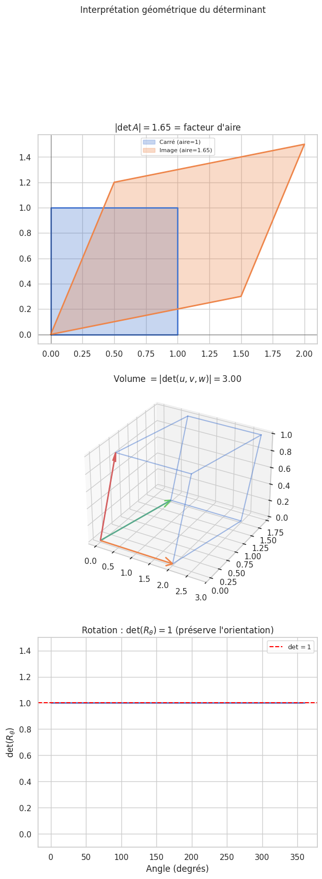
Le déterminant mesure le volume signé :

• Dimension 2 : \(|\det(u,v)|\) = aire du parallélogramme ; le signe indique l’orientation (directe ou indirecte).

• Dimension 3 : \(|\det(u,v,w)|\) = volume du parallélépipède.

• En général : \(|\det(f)|\) = facteur de dilatation des volumes par \(f\).

Si \(\det(f) > 0\) : \(f\) préserve l’orientation. Si \(\det(f) < 0\) : \(f\) renverse l’orientation.

Show code cell source

Hide code cell source

fig = plt.figure(figsize=(7, 18))

# 1. Déterminant 2D : effet d'une transformation sur un carré
ax1 = fig.add_subplot(311)
square = np.array([[0,0],[1,0],[1,1],[0,1],[0,0]])
A_shear = np.array([[1.5, 0.5], [0.3, 1.2]])
transformed_sq = (A_shear @ square.T).T

ax1.fill(square[:-1,0], square[:-1,1], alpha=0.3, color='C0', label='Carré (aire=1)')
ax1.fill(transformed_sq[:-1,0], transformed_sq[:-1,1], alpha=0.3, color='C1',
         label=f'Image (aire={abs(np.linalg.det(A_shear)):.2f})')
ax1.plot(square[:,0], square[:,1], 'C0-', lw=2)
ax1.plot(transformed_sq[:,0], transformed_sq[:,1], 'C1-', lw=2)
ax1.set(aspect='equal', title=f'$|\\det A| = {abs(np.linalg.det(A_shear)):.2f}$ = facteur d\'aire')
ax1.legend(fontsize=8)
ax1.axhline(0, color='k', lw=0.4); ax1.axvline(0, color='k', lw=0.4)

# 2. Volume du parallélépipède (3D)
ax2 = fig.add_subplot(312, projection='3d')
u = np.array([2, 0, 0])
v = np.array([0.5, 1.5, 0])
w = np.array([0.3, 0.2, 1])
volume = abs(np.linalg.det(np.column_stack([u,v,w])))
# Dessiner le parallélépipède
from itertools import combinations
vertices = np.array([a*u + b*v + c*w for a in [0,1] for b in [0,1] for c in [0,1]])
edges = [(0,1),(0,2),(0,4),(1,3),(1,5),(2,3),(2,6),(3,7),(4,5),(4,6),(5,7),(6,7)]
for i,j in edges:
    ax2.plot3D(*zip(vertices[i],vertices[j]), 'C0-', alpha=0.5)
ax2.quiver(0,0,0,*u, color='C1', lw=2, arrow_length_ratio=0.1)
ax2.quiver(0,0,0,*v, color='C2', lw=2, arrow_length_ratio=0.1)
ax2.quiver(0,0,0,*w, color='C3', lw=2, arrow_length_ratio=0.1)
ax2.set(title=f'Volume $= |\\det(u,v,w)| = {volume:.2f}$')

# 3. Stabilité du signe : rotations
angles = np.linspace(0, 2*np.pi, 100)
dets = [np.linalg.det(np.array([[np.cos(t), -np.sin(t)],
                                  [np.sin(t),  np.cos(t)]])) for t in angles]
ax3 = fig.add_subplot(313)
ax3.plot(np.degrees(angles), dets, 'C0-', lw=2)
ax3.axhline(1, color='red', ls='--', label='$\\det = 1$')
ax3.set(xlabel='Angle (degrés)', ylabel='$\\det(R_\\theta)$',
        title='Rotation : $\\det(R_\\theta) = 1$ (préserve l\'orientation)')
ax3.legend(fontsize=9)
ax3.set_ylim(-0.1, 1.5)

plt.suptitle('Interprétation géométrique du déterminant', fontsize=12, y=1.02)
plt.show()

Déterminant d’un endomorphisme

Définition 170 (Déterminant d’un endomorphisme)

Le déterminant de \(f \in \mathcal{L}(E)\) est \(\det(f) = \det(\mathrm{Mat}_\mathcal{B}(f))\) pour n’importe quelle base \(\mathcal{B}\) (bien défini car invariant par similitude).

Proposition 257

• \(f\) automorphisme \(\iff\) \(\det(f) \neq 0\)

• \(\det(g \circ f) = \det(g)\,\det(f)\)

• \(\det(\lambda\,\mathrm{id}) = \lambda^n\)

Exemple 89

• \(\det(\mathrm{id}) = 1\)

• Symétrie : \(\det = -1\) si l’espace est impair, \(\pm 1\) en général

• Homothétie \(\lambda\,\mathrm{id}\) : \(\det = \lambda^n\)

• Rotation en dimension paire : \(\det = 1\)