Fonctions usuelles

Fonctions usuelles#

La lecture d’Euler est le maître de nous tous.

Pierre-Simon de Laplace

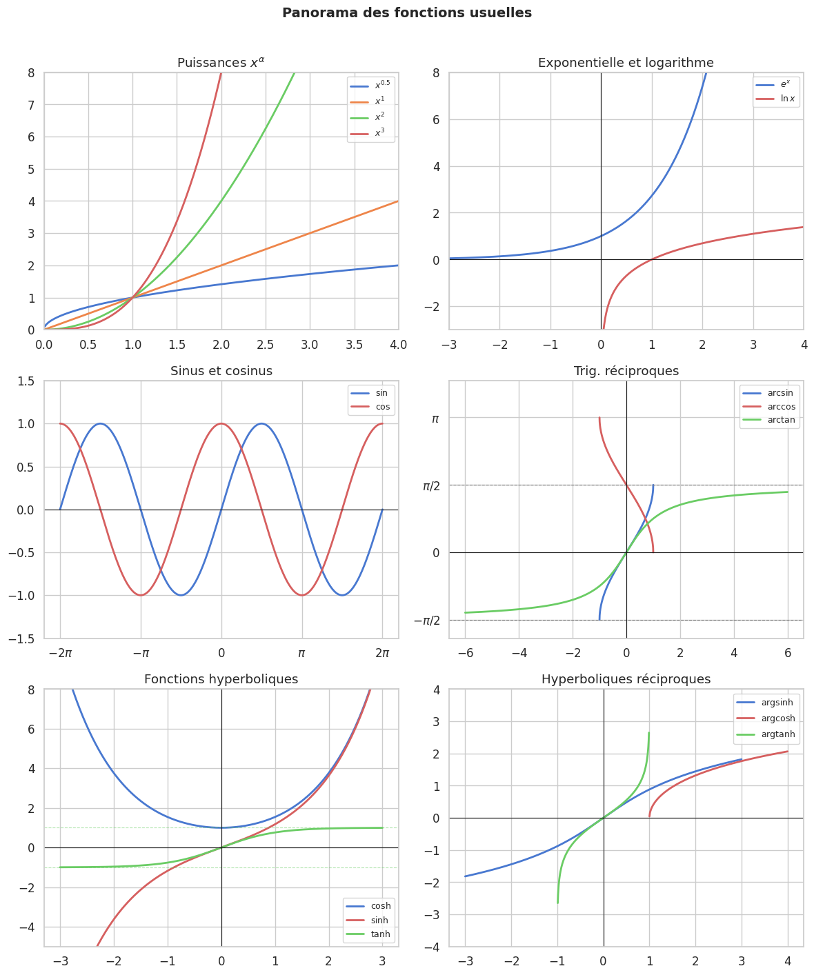
Ce chapitre rassemble les fonctions fondamentales de l’analyse : puissances, exponentielle, logarithme, fonctions trigonométriques et hyperboliques, ainsi que leurs réciproques. Ces fonctions sont les briques élémentaires à partir desquelles se construit l’essentiel de l’analyse réelle et complexe.

Fonctions puissances#

Puissances entières#

Définition 108 (Puissance entière)

Pour $n \in \mathbb{Z}$ et $x \in \mathbb{R}$ (avec $x \neq 0$ si $n < 0$) :

\[x^n = \underbrace{x \cdot x \cdots x}_{n \text{ fois}} \quad (n \geq 0), \qquad x^n = \frac{1}{x^{-n}} \quad (n < 0).\]

Par convention, $x^0 = 1$ pour tout $x \neq 0$.

Proposition 159 (Propriétés algébriques)

$\forall x, y \in \mathbb{R}^*$, $\forall m, n \in \mathbb{Z}$ :

$x^{m+n} = x^m \cdot x^n$
$x^{mn} = (x^m)^n$
$(xy)^n = x^n y^n$

Proposition 160 (Dérivée et classe)

La fonction $x \mapsto x^n$ est de classe $\mathcal{C}^\infty$ sur $\mathbb{R}$ (si $n \geq 0$) ou sur $\mathbb{R}^*$ (si $n < 0$), et

\[(x^n)' = nx^{n-1}.\]

Remarque 70

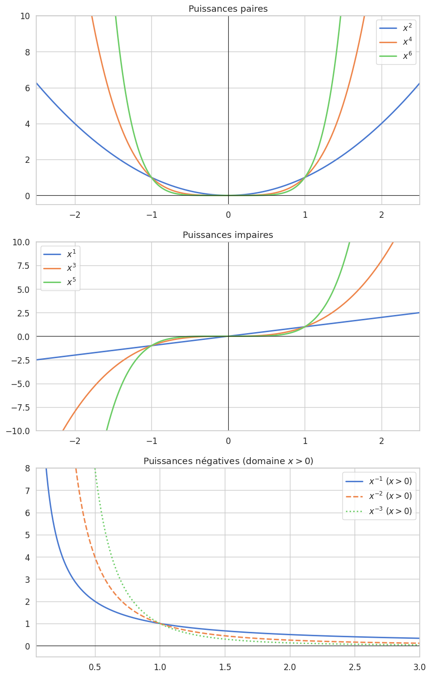
Les monômes $x \mapsto x^n$ ont des comportements très différents selon la parité de $n$ et son signe :

$n$ pair : fonction paire, minimum en 0 (si $n > 0$)
$n$ impair : fonction impaire, strictement croissante sur $\mathbb{R}$ (si $n > 0$)
$n < 0$ : pôle en 0, asymptote horizontale $y = 0$ en $\pm\infty$

_images/d51f931ed1ed89e9e627c7f0e16e71059e131e102ad39742d7560de9d02057c1.png

Puissances réelles#

Définition 109 (Puissance réelle)

Pour $x > 0$ et $\alpha \in \mathbb{R}$ :

\[x^\alpha = e^{\alpha \ln x}.\]

Pour $r = p/q \in \mathbb{Q}$ avec $q \geq 1$, cela coïncide avec $x^r = (\sqrt[q]{x})^p$.

Proposition 161

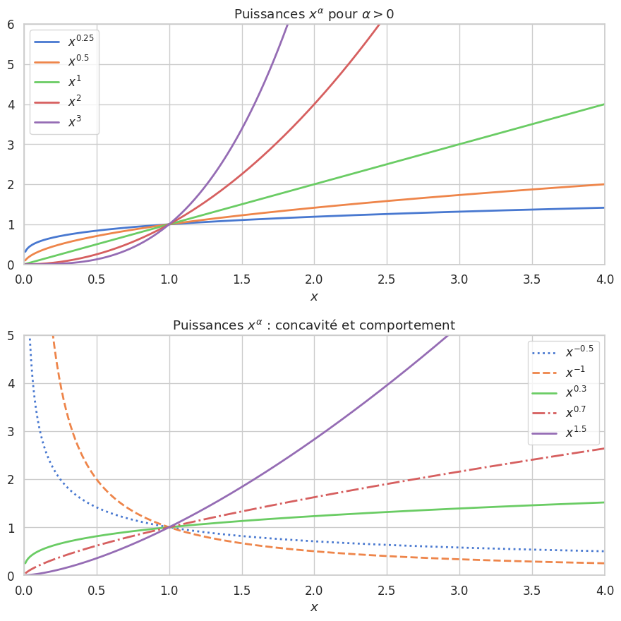
La fonction $x \mapsto x^\alpha$ est définie sur $]0, +\infty[$, de classe $\mathcal{C}^\infty$, et

\[(x^\alpha)' = \alpha x^{\alpha - 1}, \qquad (x^\alpha)'' = \alpha(\alpha-1) x^{\alpha-2}.\]

Elle est convexe si $\alpha \geq 1$ ou $\alpha \leq 0$, concave si $0 \leq \alpha \leq 1$.

Remarque 71

Le comportement en 0 et en $+\infty$ dépend du signe de $\alpha$ :

$\alpha > 0$ : $x^\alpha \to 0$ en $0^+$ et $x^\alpha \to +\infty$ en $+\infty$
$\alpha < 0$ : $x^\alpha \to +\infty$ en $0^+$ et $x^\alpha \to 0$ en $+\infty$
$\alpha = 0$ : $x^0 = 1$ (fonction constante)

_images/596d6f32386688909e5c42c36ac81dfb4539fa8f4a17304ac204d5e25b3b0a6b.png

Exponentielle et logarithme#

Le logarithme népérien#

Définition 110 (Logarithme népérien)

Le logarithme népérien est l’unique primitive de $x \mapsto 1/x$ sur $]0, +\infty[$ s’annulant en 1 :

\[\ln : \:]0, +\infty[ \to \mathbb{R}, \qquad \ln'(x) = \frac{1}{x}, \quad \ln(1) = 0.\]

Proposition 162 (Propriétés du logarithme)

$\forall x, y > 0$, $\forall \alpha \in \mathbb{R}$ :

$\ln(xy) = \ln x + \ln y$ (morphisme de $(\mathbb{R}^*_+, \cdot)$ dans $(\mathbb{R}, +)$)
$\ln\!\left(\dfrac{x}{y}\right) = \ln x - \ln y$
$\ln(x^\alpha) = \alpha \ln x$
$\ln$ est strictement croissante et concave sur $]0, +\infty[$
$\lim_{x \to 0^+} \ln x = -\infty$, $\quad \lim_{x \to +\infty} \ln x = +\infty$
$\ln$ réalise une bijection de $]0, +\infty[$ sur $\mathbb{R}$

Proof. Morphisme : Posons $g(x) = \ln(ax)$ pour $a > 0$ fixé. Alors $g'(x) = \frac{1}{x} = \ln'(x)$. Donc $g - \ln$ est constante ; en $x = 1$ : $g(1) - \ln(1) = \ln(a)$. Ainsi $\ln(ax) = \ln(a) + \ln(x)$ pour tout $x > 0$.

Concavité : $\ln''(x) = -1/x^2 < 0$.

Bijectivité : $\ln$ est continue, strictement croissante, et $\ln(2^n) = n\ln 2 \to +\infty$, $\ln(2^{-n}) \to -\infty$ : par le TVI, $\ln$ est surjective.

Proposition 163 (Inégalité fondamentale)

\[\forall x > 0, \quad \ln x \leq x - 1,\]

avec égalité si et seulement si $x = 1$.

Proof. Posons $\varphi(x) = \ln x - (x - 1)$. On a $\varphi'(x) = 1/x - 1$, qui s’annule en $x = 1$ et est positif sur $]0, 1[$ et négatif sur $]1, +\infty[$. Donc $\varphi$ est maximale en $x = 1$, avec $\varphi(1) = 0$.

L’exponentielle#

Définition 111 (Exponentielle)

La fonction exponentielle $\exp : \mathbb{R} \to \:]0, +\infty[$ est la bijection réciproque de $\ln$.

\[y = e^x \iff x = \ln y.\]

Proposition 164 (Propriétés de l’exponentielle)

$\forall x, y \in \mathbb{R}$ :

$e^{x+y} = e^x \cdot e^y$ (morphisme de $(\mathbb{R}, +)$ dans $(\mathbb{R}^*_+, \cdot)$)
$e^{-x} = \dfrac{1}{e^x}$, $\quad e^0 = 1$
$\exp' = \exp$ : l’exponentielle est sa propre dérivée
$e^x > 0$ pour tout $x$
$\exp$ est strictement croissante et convexe sur $\mathbb{R}$
$\lim_{x \to -\infty} e^x = 0$, $\quad \lim_{x \to +\infty} e^x = +\infty$

Proof. Dérivée : Par dérivation de la réciproque : $\exp'(x) = \dfrac{1}{\ln'(\exp(x))} = \dfrac{1}{1/e^x} = e^x$.

Convexité : $\exp'' = \exp > 0$.

Morphisme : $\ln(e^x \cdot e^y) = x + y = \ln(e^{x+y})$, puis injectivité de $\ln$.

Proposition 165 (Inégalité de convexité)

\[\forall x \in \mathbb{R}, \quad e^x \geq 1 + x,\]

avec égalité si et seulement si $x = 0$.

Proof. Cela résulte directement de $\ln x \leq x - 1$ en posant $x = e^t$ : $t \leq e^t - 1$, soit $e^t \geq 1 + t$. Ou directement : $\exp$ est convexe, donc son graphe est au-dessus de toute tangente ; la tangente en 0 est $y = 1 + x$.

Définition 112 (Nombre $e$)

\[e = \exp(1) = \sum_{n=0}^{+\infty} \frac{1}{n!} \approx 2{,}71828\ldots\]

Proposition 166 (Irrationalité de $e$)

Le nombre $e$ est irrationnel (et même transcendant).

Proof. Irrationalité. Par l’absurde : supposons $e = p/q$ avec $p, q \in \mathbb{N}^*$. Posons

\[N = q!\left(e - \sum_{k=0}^{q} \frac{1}{k!}\right) = q! \sum_{k=q+1}^{+\infty} \frac{1}{k!}.\]

D’une part, $N = (q-1)! p - \sum_{k=0}^{q} \frac{q!}{k!} \in \mathbb{Z}$. D’autre part, $0 < N < \sum_{j=1}^{+\infty} \frac{1}{(q+1)^j} = \frac{1}{q} \leq 1$. Contradiction : il n’existe pas d’entier dans $]0, 1[$.

Show code cell source

Hide code cell source

fig, axes = plt.subplots(3, 1, figsize=(9, 14))

# exp et ln, symétrie par rapport à y=x
x_exp = np.linspace(-3, 3, 500)
x_log = np.linspace(0.01, 6, 500)

axes[0].plot(x_exp, np.exp(x_exp), 'b-', linewidth=2.5, label='$e^x$')
axes[0].plot(x_log, np.log(x_log), 'r-', linewidth=2.5, label='$\\ln(x)$')
axes[0].plot(x_exp, x_exp, 'k--', linewidth=1, alpha=0.5, label='$y=x$')
# Tangente en 0 pour exp : y = 1 + x
axes[0].plot(x_exp, 1 + x_exp, 'b:', linewidth=1.5, alpha=0.7, label='Tangente $y=1+x$')
axes[0].axhline(0, color='k', lw=0.8)
axes[0].axvline(0, color='k', lw=0.8)
axes[0].set_xlim(-3, 4)
axes[0].set_ylim(-3, 6)
axes[0].set_title('$e^x$ et $\\ln(x)$ : fonctions réciproques\n$e^x \\geq 1+x$, $\\ln x \\leq x-1$')
axes[0].legend(fontsize=9)
axes[0].set_xlabel('$x$')

# Convexité de exp : droite reliant deux points est au-dessus du graphe
x = np.linspace(-2, 2, 500)
a, b = -1, 1.5
t = np.linspace(0, 1, 50)
axes[1].plot(x, np.exp(x), 'b-', linewidth=2.5, label='$e^x$ (convexe)')
axes[1].plot([a, b], [np.exp(a), np.exp(b)], 'r-', linewidth=2, label='Corde $[a,b]$')
axes[1].fill_between(np.linspace(a, b, 100),
                      np.exp(np.linspace(a, b, 100)),
                      np.exp(a) + (np.exp(b)-np.exp(a))/(b-a)*(np.linspace(a,b,100)-a),
                      alpha=0.15, color='red')
axes[1].scatter([a, b], [np.exp(a), np.exp(b)], color='red', s=80, zorder=5)
axes[1].axhline(0, color='k', lw=0.8)
axes[1].axvline(0, color='k', lw=0.8)
axes[1].set_xlim(-2.5, 2.5)
axes[1].set_ylim(-0.5, 8)
axes[1].set_title('Convexité de $e^x$ :\ncorde au-dessus du graphe')
axes[1].legend()
axes[1].set_xlabel('$x$')

# Croissances comparées
x = np.linspace(0.5, 8, 500)
axes[2].semilogy(x, np.log(x), 'b-', linewidth=2, label='$\\ln(x)$')
axes[2].semilogy(x, x**0.5, 'g-', linewidth=2, label='$\\sqrt{x}$')
axes[2].semilogy(x, x, 'orange', linewidth=2, label='$x$')
axes[2].semilogy(x, x**2, 'm-', linewidth=2, label='$x^2$')
axes[2].semilogy(x, np.exp(x), 'r-', linewidth=2, label='$e^x$')
axes[2].set_xlim(0.5, 8)
axes[2].set_title('Croissances comparées (échelle log)\n$\\ln \\ll x^\\alpha \\ll e^x$')
axes[2].legend(fontsize=9)
axes[2].set_xlabel('$x$')

plt.tight_layout()
plt.show()

_images/70ad9426fd853de2cd15e8ef9141f20f3071b4f62de34896e4738bd399fba627.png

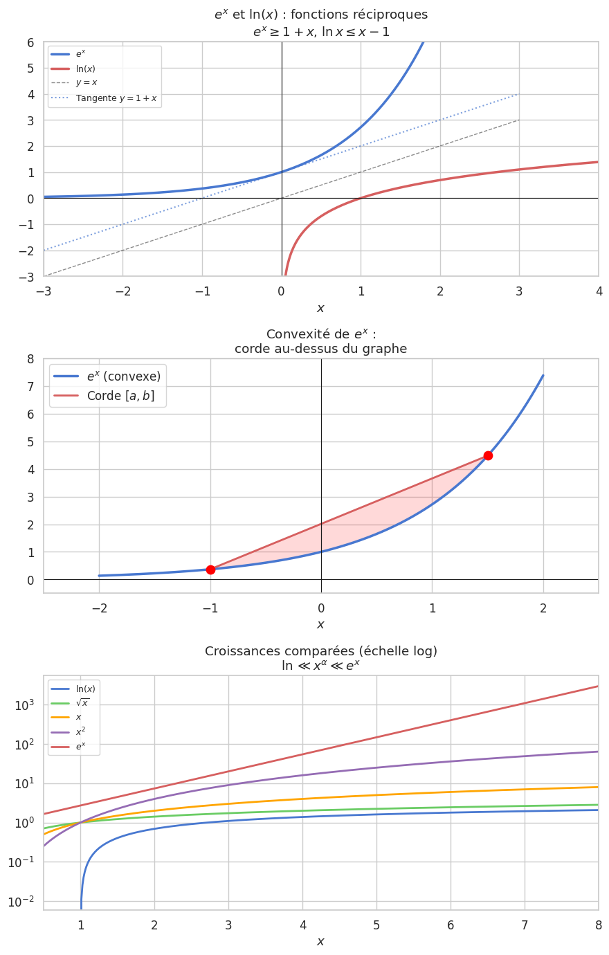
Croissances comparées#

Proposition 167 (Croissances comparées)

$\forall \alpha > 0$, $\forall \beta > 0$ :

\[\lim_{x \to +\infty} \frac{(\ln x)^\alpha}{x^\beta} = 0, \qquad \lim_{x \to +\infty} \frac{x^\alpha}{e^{\beta x}} = 0, \qquad \lim_{x \to 0^+} x^\alpha |\ln x|^\beta = 0.\]

Proof. $\frac{\ln x}{x^\beta} \to 0$ : On se ramène à $\frac{\ln x}{\sqrt{x}} \to 0$ par $\frac{(\ln x)^\alpha}{x^\beta} = \left(\frac{\ln x}{x^{\beta/\alpha}}\right)^\alpha$. Posons $x = e^t$ ($t \to +\infty$) : $\frac{\ln x}{\sqrt{x}} = \frac{t}{e^{t/2}} \leq \frac{2t}{t^2} = \frac{2}{t} \to 0$ (car $e^{t/2} \geq t^2/2$ pour $t$ assez grand).

$\frac{x^\alpha}{e^{\beta x}} \to 0$ : Par le DL, $e^{\beta x} \geq \frac{(\beta x)^n}{n!}$ pour tout $n$. Choisir $n > \alpha$.

En 0 : Poser $t = -\ln x \to +\infty$ : $x^\alpha |\ln x|^\beta = e^{-\alpha t} t^\beta \to 0$.

Remarque 72

Ces résultats se résument par la hiérarchie :

\[\ln x \ll x^\alpha \ll e^x \quad (x \to +\infty), \quad \forall \alpha > 0.\]

Plus généralement, pour $0 < \alpha < \beta$ : $x^\alpha \ll x^\beta$ en $+\infty$.

Exponentielle de base $a$#

Définition 113

Pour $a > 0$, $a \neq 1$ et $x \in \mathbb{R}$ :

\[a^x = e^{x \ln a}, \qquad \log_a x = \frac{\ln x}{\ln a} \quad (x > 0).\]

Proposition 168

$(a^x)' = (\ln a)\, a^x$ et $(\log_a x)' = \dfrac{1}{x \ln a}$. Si $a > 1$ : $a^x$ est croissante ; si $0 < a < 1$ : $a^x$ est décroissante.

Fonctions trigonométriques#

Le cercle trigonométrique#

Les fonctions $\cos$ et $\sin$ sont définies géométriquement par les coordonnées du point de $\mathbb{R}^2$ situé sur le cercle unité à l’angle $\theta$ du demi-axe $Ox$ positif. Analytiquement, elles se définissent par leurs développements en série entière :

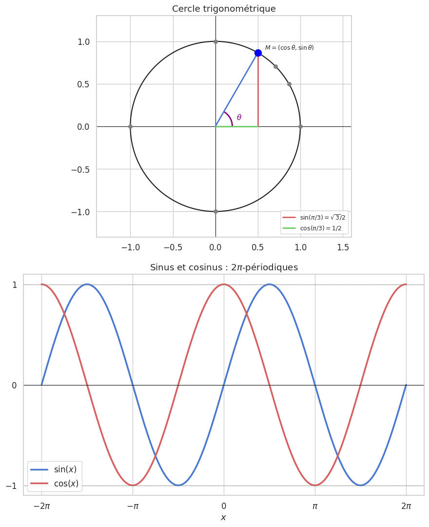
\[\cos x = \sum_{n=0}^{+\infty} \frac{(-1)^n x^{2n}}{(2n)!}, \qquad \sin x = \sum_{n=0}^{+\infty} \frac{(-1)^n x^{2n+1}}{(2n+1)!}.\]

_images/484cec897151de969e8f66b78fd1818a446514e22c50cc028120296272e3f3fa.png

Propriétés fondamentales#

Proposition 169 (Propriétés de $\sin$ et $\cos$)

$\sin$ et $\cos$ sont de classe $\mathcal{C}^\infty$ sur $\mathbb{R}$, à valeurs dans $[-1, 1]$, $2\pi$-périodiques
$\sin' = \cos$ et $\cos' = -\sin$
$\sin$ est impaire, $\cos$ est paire
$\forall x \in \mathbb{R}$, $\cos^2 x + \sin^2 x = 1$ (relation de Pythagore)
$\sin$ est croissante sur $[-\pi/2, \pi/2]$, $\cos$ est décroissante sur $[0, \pi]$

Proposition 170 (Formules d’addition)

\[\cos(a + b) = \cos a \cos b - \sin a \sin b\]

\[\sin(a + b) = \sin a \cos b + \cos a \sin b\]

Proof. Ces formules se démontrent analytiquement en développant $e^{i(a+b)} = e^{ia} e^{ib}$ (formule d’Euler : $e^{i\theta} = \cos\theta + i\sin\theta$) et en identifiant parties réelle et imaginaire. Parties réelles : $\cos(a+b) = \cos a \cos b - \sin a \sin b$. Parties imaginaires : $\sin(a+b) = \sin a \cos b + \cos a \sin b$.

Proposition 171 (Formules dérivées)

Duplication :

\[\cos(2a) = \cos^2 a - \sin^2 a = 2\cos^2 a - 1 = 1 - 2\sin^2 a\]

\[\sin(2a) = 2\sin a \cos a\]

Linéarisation :

\[\cos^2 a = \frac{1 + \cos(2a)}{2}, \qquad \sin^2 a = \frac{1 - \cos(2a)}{2}\]

Produit en somme :

\[\cos a \cos b = \frac{\cos(a-b) + \cos(a+b)}{2}, \qquad \sin a \sin b = \frac{\cos(a-b) - \cos(a+b)}{2}\]

\[\sin a \cos b = \frac{\sin(a+b) + \sin(a-b)}{2}\]

Somme en produit :

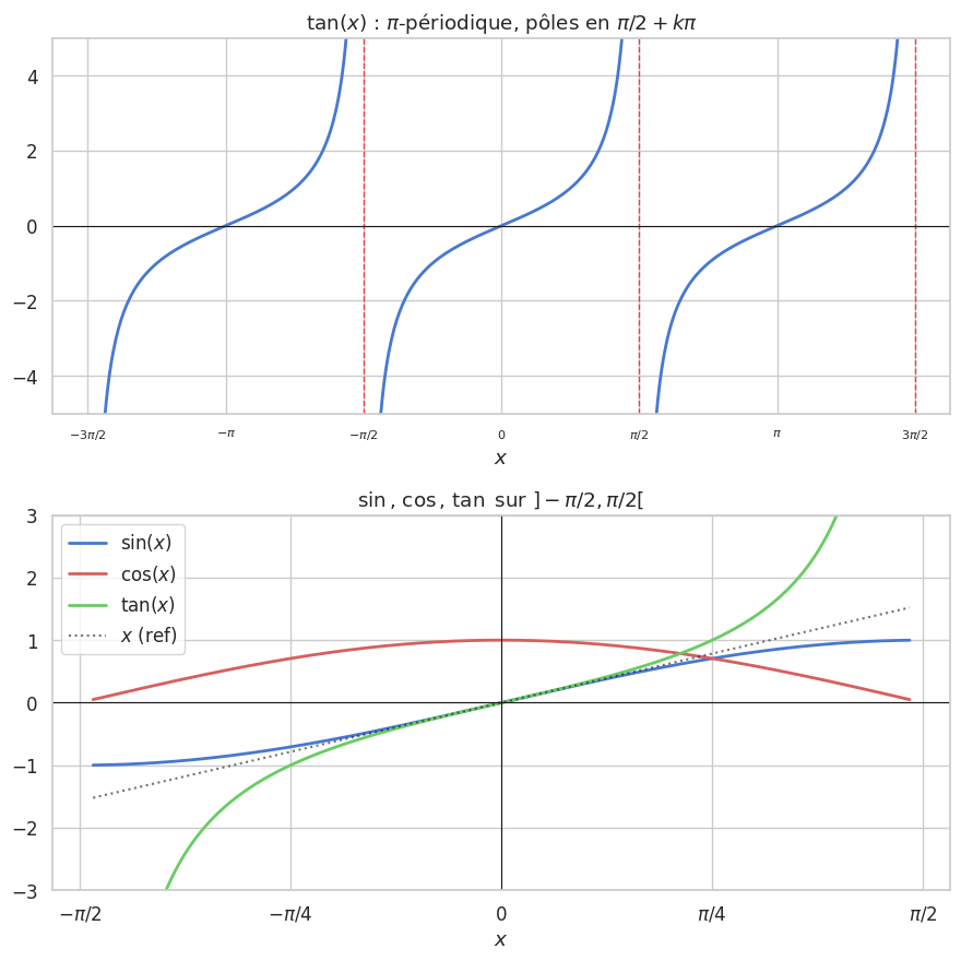
\[\cos p + \cos q = 2\cos\frac{p+q}{2}\cos\frac{p-q}{2}, \qquad \sin p + \sin q = 2\sin\frac{p+q}{2}\cos\frac{p-q}{2}\]

Proposition 172 (Limite fondamentale)

\[\lim_{x \to 0} \frac{\sin x}{x} = 1.\]

Plus précisément : $\sin x = x - \dfrac{x^3}{6} + o(x^3)$.

Proof. Par le DL de $\sin$ (voir chapitre 12) : $\sin x = x - x^3/6 + O(x^5)$, donc $\frac{\sin x}{x} = 1 - x^2/6 + O(x^4) \to 1$.

Géométriquement, l’aire du secteur angulaire vaut $x/2$, comprise entre l’aire du triangle intérieur ($\sin x \cos x / 2$) et celle du triangle extérieur ($\tan x / 2$), ce qui donne $\cos x \leq \frac{\sin x}{x} \leq \frac{1}{\cos x}$ pour $x \in ]0, \pi/2[$, et on conclut par le théorème des gendarmes.

Valeurs remarquables#

Remarque 73

Le tableau suivant est indispensable :

$x$	$0$	$\pi/6$	$\pi/4$	$\pi/3$	$\pi/2$
$\cos x$	$1$	$\frac{\sqrt{3}}{2}$	$\frac{\sqrt{2}}{2}$	$\frac{1}{2}$	$0$
$\sin x$	$0$	$\frac{1}{2}$	$\frac{\sqrt{2}}{2}$	$\frac{\sqrt{3}}{2}$	$1$
$\tan x$	$0$	$\frac{1}{\sqrt{3}}$	$1$	$\sqrt{3}$	$-$

Tangente#

Définition 114 (Tangente)

\[\tan x = \frac{\sin x}{\cos x}, \quad \text{définie sur } \mathbb{R} \setminus \left\{\frac{\pi}{2} + k\pi,\; k \in \mathbb{Z}\right\}.\]

Proposition 173

$\tan$ est $\pi$-périodique, impaire, de classe $\mathcal{C}^\infty$ sur son domaine
$\tan' = 1 + \tan^2 = \dfrac{1}{\cos^2}$
$\tan$ est strictement croissante et convexe sur $]0, \pi/2[$, strictement concave sur $]-\pi/2, 0[$
$\tan$ réalise une bijection de $]-\tfrac{\pi}{2}, \tfrac{\pi}{2}[$ sur $\mathbb{R}$
$\tan(a+b) = \dfrac{\tan a + \tan b}{1 - \tan a \tan b}$ (quand $\tan a \tan b \neq 1$)

Définition 115 (Formules du demi-angle (substitution $t = \tan(x/2)$))

Pour $x \notin \pi + 2\pi\mathbb{Z}$, en posant $t = \tan(x/2)$ :

\[\cos x = \frac{1-t^2}{1+t^2}, \qquad \sin x = \frac{2t}{1+t^2}, \qquad \tan x = \frac{2t}{1-t^2}.\]

Proof. $\cos x = \cos^2(x/2) - \sin^2(x/2) = \cos^2(x/2)(1 - \tan^2(x/2)) = \frac{1 - t^2}{1+t^2}$ en divisant par $\cos^2(x/2) + \sin^2(x/2)$.

_images/0ddec250e5129f4a85230542f5f305d88c334558e456d80ca77eba901630c73c.png

Fonctions trigonométriques réciproques#

Arcsinus#

Définition 116 (Arcsinus)

$\arcsin : [-1, 1] \to [-\frac{\pi}{2}, \frac{\pi}{2}]$ est la bijection réciproque de $\sin\!\restriction_{[-\pi/2, \pi/2]}$.

\[y = \arcsin x \iff x = \sin y \text{ et } y \in \left[-\frac{\pi}{2}, \frac{\pi}{2}\right].\]

Proposition 174

$\arcsin$ est impaire, strictement croissante, de classe $\mathcal{C}^\infty$ sur $]-1, 1[$
$\arcsin'(x) = \dfrac{1}{\sqrt{1 - x^2}}$ pour $x \in \:]-1, 1[$
$\arcsin(1) = \pi/2$, $\arcsin(-1) = -\pi/2$
DL en 0 : $\arcsin x = x + \dfrac{x^3}{6} + \dfrac{3x^5}{40} + O(x^7)$

Proof. Par dérivation de la réciproque : $\arcsin'(x) = \dfrac{1}{\sin'(\arcsin x)} = \dfrac{1}{\cos(\arcsin x)}$. Or $\cos(\arcsin x) = \sqrt{1 - \sin^2(\arcsin x)} = \sqrt{1 - x^2} > 0$ car $\arcsin x \in ]-\pi/2, \pi/2[$.

Arccosinus#

Définition 117 (Arccosinus)

$\arccos : [-1, 1] \to [0, \pi]$ est la bijection réciproque de $\cos\!\restriction_{[0,\pi]}$.

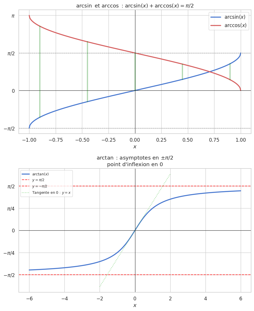
Proposition 175

$\arccos$ est strictement décroissante, de classe $\mathcal{C}^\infty$ sur $]-1, 1[$
$\arccos'(x) = \dfrac{-1}{\sqrt{1 - x^2}}$ pour $x \in \:]-1, 1[$
$\forall x \in [-1, 1]$, $\arcsin x + \arccos x = \dfrac{\pi}{2}$

Proof. Relation complémentaire : Posons $g(x) = \arcsin x + \arccos x$. Alors $g'(x) = 1/\sqrt{1-x^2} - 1/\sqrt{1-x^2} = 0$, donc $g$ est constante. En $x = 0$ : $g(0) = 0 + \pi/2$.

Arctangente#

Définition 118 (Arctangente)

$\arctan : \mathbb{R} \to ]-\frac{\pi}{2}, \frac{\pi}{2}[$ est la bijection réciproque de $\tan\!\restriction_{]-\pi/2, \pi/2[}$.

Proposition 176

$\arctan$ est impaire, strictement croissante, de classe $\mathcal{C}^\infty$ sur $\mathbb{R}$
$\arctan'(x) = \dfrac{1}{1 + x^2}$
$\lim_{x \to +\infty} \arctan x = \dfrac{\pi}{2}$, $\quad \lim_{x \to -\infty} \arctan x = -\dfrac{\pi}{2}$
$\arctan$ est concave sur $\mathbb{R}^+$ et convexe sur $\mathbb{R}^-$, point d’inflexion en 0
DL en 0 : $\arctan x = x - \dfrac{x^3}{3} + \dfrac{x^5}{5} - \cdots = \sum_{n=0}^{+\infty} \dfrac{(-1)^n x^{2n+1}}{2n+1}$ (pour $|x| \leq 1$)

Proof. $\arctan'(x) = \dfrac{1}{\tan'(\arctan x)} = \dfrac{1}{1 + \tan^2(\arctan x)} = \dfrac{1}{1 + x^2}$.

DL : $\dfrac{1}{1+x^2} = \sum_{n=0}^{N} (-1)^n x^{2n} + O(x^{2N+2})$ par la série géométrique. On intègre terme à terme (justifié par convergence uniforme sur $[-r, r]$, $r < 1$).

Remarque 74

La formule de Leibniz : $\dfrac{\pi}{4} = \arctan 1 = \sum_{n=0}^{+\infty} \dfrac{(-1)^n}{2n+1} = 1 - \dfrac{1}{3} + \dfrac{1}{5} - \cdots$

La convergence est très lente. En pratique on utilise $\dfrac{\pi}{4} = \arctan\!\tfrac{1}{2} + \arctan\!\tfrac{1}{3}$ (formule de Machin) pour converger plus vite.

_images/f6c0de346f250ccf6905dc00bb0963fb419903a2eb2d5360197cbf123cf2198b.png

Fonctions hyperboliques#

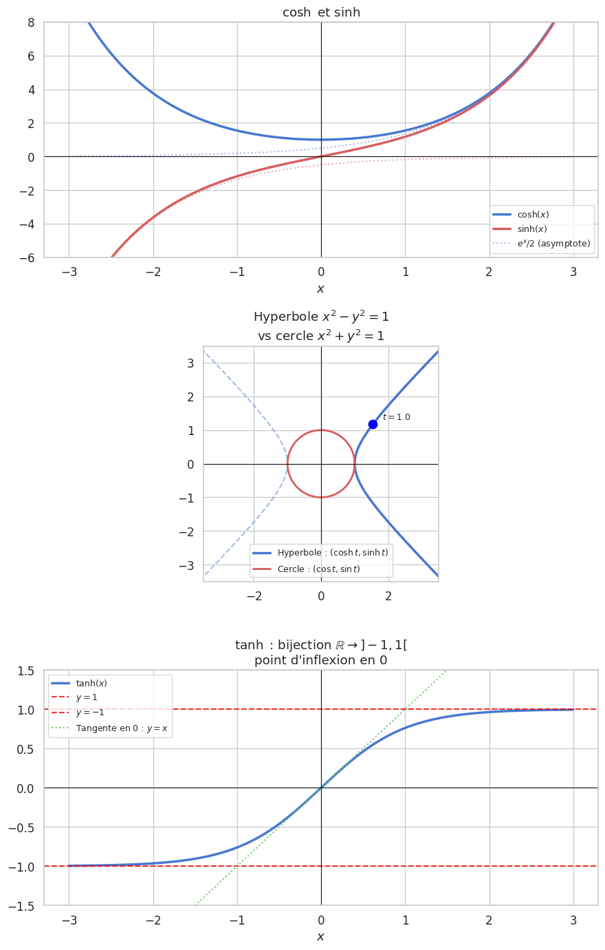
Les fonctions hyperboliques sont les analogues réels des fonctions trigonométriques, mais pour l’hyperbole $x^2 - y^2 = 1$ au lieu du cercle $x^2 + y^2 = 1$.

Cosinus et sinus hyperboliques#

Définition 119 (Cosinus et sinus hyperboliques)

\[\cosh x = \frac{e^x + e^{-x}}{2}, \qquad \sinh x = \frac{e^x - e^{-x}}{2}.\]

Remarque 75

Ces fonctions décomposent l’exponentielle en parties paire et impaire :

\[e^x = \cosh x + \sinh x, \qquad e^{-x} = \cosh x - \sinh x.\]

Le point $(\cosh t, \sinh t)$ décrit la branche droite de l’hyperbole $x^2 - y^2 = 1$, de même que $(\cos t, \sin t)$ décrit le cercle unité. L’angle $t$ est ici l’aire du secteur hyperbolique (cf. la signification paramétrique).

Proposition 177 (Propriétés de $\cosh$ et $\sinh$)

$\cosh$ est paire, $\sinh$ est impaire
$\cosh' = \sinh$ et $\sinh' = \cosh$
$\cosh^2 x - \sinh^2 x = 1$ (identité fondamentale, analogue de $\cos^2 + \sin^2 = 1$)
$\cosh x \geq 1$ pour tout $x$, avec égalité uniquement en $x = 0$
$\cosh$ est convexe (minimum en 0), $\sinh$ est convexe sur $\mathbb{R}^+$ et concave sur $\mathbb{R}^-$
$\sinh$ est une bijection strictement croissante de $\mathbb{R}$ sur $\mathbb{R}$

Proof. Identité fondamentale :

\[\cosh^2 x - \sinh^2 x = \frac{(e^x + e^{-x})^2 - (e^x - e^{-x})^2}{4} = \frac{4}{4} = 1.\]

$\cosh x \geq 1$ : Par l’inégalité arithmético-géométrique : $\dfrac{e^x + e^{-x}}{2} \geq \sqrt{e^x \cdot e^{-x}} = 1$.

Convexité de $\cosh$ : $\cosh'' = \cosh > 0$.

Proposition 178 (Formules d’addition)

\[\cosh(a + b) = \cosh a \cosh b + \sinh a \sinh b\]

\[\sinh(a + b) = \sinh a \cosh b + \cosh a \sinh b\]

Proof. Développer $\cosh a \cosh b + \sinh a \sinh b = \frac{(e^a+e^{-a})(e^b+e^{-b}) + (e^a-e^{-a})(e^b-e^{-b})}{4} = \frac{2e^{a+b}+2e^{-(a+b)}}{4} = \cosh(a+b)$.

Proposition 179 (Formules de duplication)

\[\cosh(2x) = 2\cosh^2 x - 1 = 1 + 2\sinh^2 x, \qquad \sinh(2x) = 2\sinh x \cosh x.\]

Tangente hyperbolique#

Définition 120 (Tangente hyperbolique)

\[\tanh x = \frac{\sinh x}{\cosh x} = \frac{e^x - e^{-x}}{e^x + e^{-x}} = 1 - \frac{2}{e^{2x}+1}.\]

Proposition 180

$\tanh$ est impaire, de classe $\mathcal{C}^\infty$, strictement croissante sur $\mathbb{R}$
$\tanh' = \dfrac{1}{\cosh^2} = 1 - \tanh^2$
$\tanh$ est une bijection de $\mathbb{R}$ sur $]-1, 1[$
$\lim_{x \to \pm\infty} \tanh x = \pm 1$ : asymptotes horizontales $y = \pm 1$
$\tanh$ est concave sur $\mathbb{R}^+$, point d’inflexion en 0

Show code cell source

Hide code cell source

fig, axes = plt.subplots(3, 1, figsize=(9, 14))

x = np.linspace(-3, 3, 500)

# cosh et sinh
axes[0].plot(x, np.cosh(x), 'b-', linewidth=2.5, label='$\\cosh(x)$')
axes[0].plot(x, np.sinh(x), 'r-', linewidth=2.5, label='$\\sinh(x)$')
axes[0].plot(x, np.exp(x)/2, 'b:', lw=1.5, alpha=0.5, label='$e^x/2$ (asymptote)')
axes[0].plot(x, -np.exp(-x)/2, 'r:', lw=1.5, alpha=0.5)
axes[0].axhline(0, color='k', lw=0.8)
axes[0].axvline(0, color='k', lw=0.8)
axes[0].set_ylim(-6, 8)
axes[0].set_title('$\\cosh$ et $\\sinh$')
axes[0].legend(fontsize=9)
axes[0].set_xlabel('$x$')

# Hyperbole et cercle
t = np.linspace(-2.5, 2.5, 400)
axes[1].plot(np.cosh(t), np.sinh(t), 'b-', lw=2.5, label='Hyperbole : $(\\cosh t, \\sinh t)$')
axes[1].plot(-np.cosh(t), np.sinh(t), 'b--', lw=1.5, alpha=0.5)
theta = np.linspace(0, 2*np.pi, 400)
axes[1].plot(np.cos(theta), np.sin(theta), 'r-', lw=2, label='Cercle : $(\\cos t, \\sin t)$')
# Point particulier
t0 = 1.0
axes[1].scatter([np.cosh(t0)], [np.sinh(t0)], color='blue', s=80, zorder=5)
axes[1].annotate(f'$t={t0}$', (np.cosh(t0), np.sinh(t0)),
                  xytext=(10, 5), textcoords='offset points', fontsize=9)
axes[1].axhline(0, color='k', lw=0.8)
axes[1].axvline(0, color='k', lw=0.8)
axes[1].set_aspect('equal')
axes[1].set_xlim(-3.5, 3.5)
axes[1].set_ylim(-3.5, 3.5)
axes[1].set_title('Hyperbole $x^2-y^2=1$\nvs cercle $x^2+y^2=1$')
axes[1].legend(fontsize=9)

# tanh
axes[2].plot(x, np.tanh(x), 'b-', linewidth=2.5, label='$\\tanh(x)$')
axes[2].axhline(1, color='red', ls='--', lw=1.5, alpha=0.8, label='$y=1$')
axes[2].axhline(-1, color='red', ls='--', lw=1.5, alpha=0.8, label='$y=-1$')
# Tangente en 0 : y = x (car tanh'(0)=1)
x_tan0 = np.linspace(-1.5, 1.5, 100)
axes[2].plot(x_tan0, x_tan0, 'g:', lw=1.5, label="Tangente en $0$ : $y=x$")
axes[2].axhline(0, color='k', lw=0.8)
axes[2].axvline(0, color='k', lw=0.8)
axes[2].set_ylim(-1.5, 1.5)
axes[2].set_title('$\\tanh$ : bijection $\\mathbb{R} \\to ]-1,1[$\npoint d\'inflexion en 0')
axes[2].legend(fontsize=9)
axes[2].set_xlabel('$x$')

plt.tight_layout()
plt.show()

_images/e7abc92d5791e5a8ce092a8051662853e8d8156d654bbae8774c72a3c4f88306.png

Analogie trigonométrique/hyperbolique#

Remarque 76

Le parallèle entre fonctions circulaires et hyperboliques est frappant :

Circulaire	Hyperbolique
$\cos^2 + \sin^2 = 1$	$\cosh^2 - \sinh^2 = 1$
$\cos' = -\sin$	$\cosh' = \sinh$
$\sin' = \cos$	$\sinh' = \cosh$
Cercle $x^2+y^2=1$	Hyperbole $x^2-y^2=1$
$e^{ix} = \cos x + i\sin x$	$e^x = \cosh x + \sinh x$

La formule d’Osborn permet de passer d’une identité trigonométrique à son analogue hyperbolique : remplacer $\sin$ par $i\sinh$ (ou, pratiquement, changer le signe de chaque produit de deux $\sinh$).

Fonctions hyperboliques réciproques#

$\text{argsinh}$#

Définition 121

$\text{argsinh} : \mathbb{R} \to \mathbb{R}$ est la bijection réciproque de $\sinh$.

Proposition 181

\[\text{argsinh}(x) = \ln\!\left(x + \sqrt{x^2 + 1}\right), \qquad \text{argsinh}'(x) = \frac{1}{\sqrt{x^2 + 1}}.\]

Proof. Expression logarithmique : $y = \text{argsinh}(x)$ signifie $x = \sinh y = (e^y - e^{-y})/2$. Posons $t = e^y > 0$ : $t^2 - 2xt - 1 = 0$, d’où $t = x + \sqrt{x^2+1}$ (seule racine positive). Donc $y = \ln(x + \sqrt{x^2+1})$.

Dérivée : $\text{argsinh}'(x) = 1/\sinh'(\text{argsinh}(x)) = 1/\cosh(\text{argsinh}(x)) = 1/\sqrt{1 + \sinh^2(\text{argsinh}(x))} = 1/\sqrt{1+x^2}$.

$\text{argcosh}$#

Définition 122

$\text{argcosh} : [1, +\infty[ \to [0, +\infty[$ est la bijection réciproque de $\cosh\!\restriction_{[0,+\infty[}$.

Proposition 182

\[\text{argcosh}(x) = \ln\!\left(x + \sqrt{x^2 - 1}\right), \qquad \text{argcosh}'(x) = \frac{1}{\sqrt{x^2 - 1}} \quad (x > 1).\]

Proof. $x = \cosh y = (e^y + e^{-y})/2$ avec $y \geq 0$. Posant $t = e^y \geq 1$ : $t^2 - 2xt + 1 = 0$, d’où $t = x + \sqrt{x^2-1}$ (la racine $\geq 1$). Donc $y = \ln(x + \sqrt{x^2-1})$.

$\text{argtanh}$#

Définition 123

$\text{argtanh} : ]-1, 1[ \to \mathbb{R}$ est la bijection réciproque de $\tanh$.

Proposition 183

\[\text{argtanh}(x) = \frac{1}{2}\ln\frac{1+x}{1-x}, \qquad \text{argtanh}'(x) = \frac{1}{1 - x^2}.\]

Proof. $x = \tanh y$ implique $e^{2y} = (1+x)/(1-x)$, donc $y = \frac{1}{2}\ln\frac{1+x}{1-x}$.

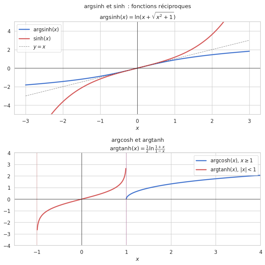
_images/df1ac351163239ca0df2783957e5bfa82c780c089bbb2d75221b39132a57d420.png

Tableau récapitulatif des dérivées#

Remarque 77

Ce tableau est à connaître absolument.

$f(x)$	$f'(x)$	Domaine
$x^n$ ($n \in \mathbb{Z}$)	$nx^{n-1}$	$\mathbb{R}$ (ou $\mathbb{R}^*$ si $n < 0$)
$x^\alpha$ ($\alpha \in \mathbb{R}$)	$\alpha x^{\alpha - 1}$	$]0, +\infty[$
$e^x$	$e^x$	$\mathbb{R}$
$a^x$ ($a > 0$)	$(\ln a)\, a^x$	$\mathbb{R}$
$\ln x$	$\dfrac{1}{x}$	$]0, +\infty[$
$\log_a x$ ($a>0, a\neq 1$)	$\dfrac{1}{x\ln a}$	$]0, +\infty[$
$\sin x$	$\cos x$	$\mathbb{R}$
$\cos x$	$-\sin x$	$\mathbb{R}$
$\tan x$	$\dfrac{1}{\cos^2 x} = 1 + \tan^2 x$	$\mathbb{R} \setminus \{\frac{\pi}{2} + k\pi\}$
$\arcsin x$	$\dfrac{1}{\sqrt{1-x^2}}$	$]-1, 1[$
$\arccos x$	$\dfrac{-1}{\sqrt{1-x^2}}$	$]-1, 1[$
$\arctan x$	$\dfrac{1}{1+x^2}$	$\mathbb{R}$
$\cosh x$	$\sinh x$	$\mathbb{R}$
$\sinh x$	$\cosh x$	$\mathbb{R}$
$\tanh x$	$\dfrac{1}{\cosh^2 x} = 1 - \tanh^2 x$	$\mathbb{R}$
$\text{argsinh}\, x$	$\dfrac{1}{\sqrt{x^2+1}}$	$\mathbb{R}$
$\text{argcosh}\, x$	$\dfrac{1}{\sqrt{x^2-1}}$	$]1, +\infty[$
$\text{argtanh}\, x$	$\dfrac{1}{1-x^2}$	$]-1, 1[$

Primitives usuelles#

Remarque 78

Le tableau suivant liste les primitives à connaître, complémentaire du tableau des dérivées.

$f(x)$	$F(x)$ (primitive)	Conditions
$x^n$ ($n \neq -1$)	$\dfrac{x^{n+1}}{n+1}$	$\mathbb{R}$ si $n \in \mathbb{N}$, $\mathbb{R}^*$ sinon
$\dfrac{1}{x}$	$\ln	x
$e^x$	$e^x$	$\mathbb{R}$
$\cos x$	$\sin x$	$\mathbb{R}$
$\sin x$	$-\cos x$	$\mathbb{R}$
$\dfrac{1}{\cos^2 x}$	$\tan x$	$x \neq \pi/2 + k\pi$
$\dfrac{1}{1+x^2}$	$\arctan x$	$\mathbb{R}$
$\dfrac{1}{\sqrt{1-x^2}}$	$\arcsin x$	$]-1,1[$
$\dfrac{1}{\sqrt{x^2+1}}$	$\text{argsinh}\, x$	$\mathbb{R}$
$\dfrac{1}{\sqrt{x^2-1}}$	$\text{argcosh}\, x$	$]1,+\infty[$
$\dfrac{1}{1-x^2}$	$\text{argtanh}\, x$	$]-1,1[$
$\cosh x$	$\sinh x$	$\mathbb{R}$
$\sinh x$	$\cosh x$	$\mathbb{R}$

_images/faf45b76ef77f71702aa165daa83dcdc97e8ceaaf38f067a54897b7317d3f16f.png

\(x\)	\(0\)	\(\pi/6\)	\(\pi/4\)	\(\pi/3\)	\(\pi/2\)
\(\cos x\)	\(1\)	\(\frac{\sqrt{3}}{2}\)	\(\frac{\sqrt{2}}{2}\)	\(\frac{1}{2}\)	\(0\)
\(\sin x\)	\(0\)	\(\frac{1}{2}\)	\(\frac{\sqrt{2}}{2}\)	\(\frac{\sqrt{3}}{2}\)	\(1\)
\(\tan x\)	\(0\)	\(\frac{1}{\sqrt{3}}\)	\(1\)	\(\sqrt{3}\)	\(-\)

Circulaire	Hyperbolique
\(\cos^2 + \sin^2 = 1\)	\(\cosh^2 - \sinh^2 = 1\)
\(\cos' = -\sin\)	\(\cosh' = \sinh\)
\(\sin' = \cos\)	\(\sinh' = \cosh\)
Cercle \(x^2+y^2=1\)	Hyperbole \(x^2-y^2=1\)
\(e^{ix} = \cos x + i\sin x\)	\(e^x = \cosh x + \sinh x\)

\(f(x)\)	\(f'(x)\)	Domaine
\(x^n\) (\(n \in \mathbb{Z}\))	\(nx^{n-1}\)	\(\mathbb{R}\) (ou \(\mathbb{R}^*\) si \(n < 0\))
\(x^\alpha\) (\(\alpha \in \mathbb{R}\))	\(\alpha x^{\alpha - 1}\)	\(]0, +\infty[\)
\(e^x\)	\(e^x\)	\(\mathbb{R}\)
\(a^x\) (\(a > 0\))	\((\ln a)\, a^x\)	\(\mathbb{R}\)
\(\ln x\)	\(\dfrac{1}{x}\)	\(]0, +\infty[\)
\(\log_a x\) (\(a>0, a\neq 1\))	\(\dfrac{1}{x\ln a}\)	\(]0, +\infty[\)
\(\sin x\)	\(\cos x\)	\(\mathbb{R}\)
\(\cos x\)	\(-\sin x\)	\(\mathbb{R}\)
\(\tan x\)	\(\dfrac{1}{\cos^2 x} = 1 + \tan^2 x\)	\(\mathbb{R} \setminus \{\frac{\pi}{2} + k\pi\}\)
\(\arcsin x\)	\(\dfrac{1}{\sqrt{1-x^2}}\)	\(]-1, 1[\)
\(\arccos x\)	\(\dfrac{-1}{\sqrt{1-x^2}}\)	\(]-1, 1[\)
\(\arctan x\)	\(\dfrac{1}{1+x^2}\)	\(\mathbb{R}\)
\(\cosh x\)	\(\sinh x\)	\(\mathbb{R}\)
\(\sinh x\)	\(\cosh x\)	\(\mathbb{R}\)
\(\tanh x\)	\(\dfrac{1}{\cosh^2 x} = 1 - \tanh^2 x\)	\(\mathbb{R}\)
\(\text{argsinh}\, x\)	\(\dfrac{1}{\sqrt{x^2+1}}\)	\(\mathbb{R}\)
\(\text{argcosh}\, x\)	\(\dfrac{1}{\sqrt{x^2-1}}\)	\(]1, +\infty[\)
\(\text{argtanh}\, x\)	\(\dfrac{1}{1-x^2}\)	\(]-1, 1[\)

\(f(x)\)	\(F(x)\) (primitive)	Conditions
\(x^n\) (\(n \neq -1\))	\(\dfrac{x^{n+1}}{n+1}\)	\(\mathbb{R}\) si \(n \in \mathbb{N}\), \(\mathbb{R}^*\) sinon
\(\dfrac{1}{x}\)	$\ln	x
\(e^x\)	\(e^x\)	\(\mathbb{R}\)
\(\cos x\)	\(\sin x\)	\(\mathbb{R}\)
\(\sin x\)	\(-\cos x\)	\(\mathbb{R}\)
\(\dfrac{1}{\cos^2 x}\)	\(\tan x\)	\(x \neq \pi/2 + k\pi\)
\(\dfrac{1}{1+x^2}\)	\(\arctan x\)	\(\mathbb{R}\)
\(\dfrac{1}{\sqrt{1-x^2}}\)	\(\arcsin x\)	\(]-1,1[\)
\(\dfrac{1}{\sqrt{x^2+1}}\)	\(\text{argsinh}\, x\)	\(\mathbb{R}\)
\(\dfrac{1}{\sqrt{x^2-1}}\)	\(\text{argcosh}\, x\)	\(]1,+\infty[\)
\(\dfrac{1}{1-x^2}\)	\(\text{argtanh}\, x\)	\(]-1,1[\)
\(\cosh x\)	\(\sinh x\)	\(\mathbb{R}\)
\(\sinh x\)	\(\cosh x\)	\(\mathbb{R}\)