Calcul intégral

Il me semble que la notion d’intégrale est restée trop étrangère à beaucoup de ceux qui auraient eu besoin de s’en servir.

Henri Lebesgue

L’intégrale généralise la notion d’aire sous une courbe. Après avoir posé les fondements de l’intégrale de Riemann, ce chapitre développe les techniques de calcul — intégration par parties, changement de variable, fractions rationnelles — et étend la théorie aux intégrales impropres, essentielles en probabilités et en physique.

Show code cell source

Hide code cell source

import numpy as np
import matplotlib.pyplot as plt
import seaborn as sns
import math
from scipy import integrate

sns.set_theme(style="whitegrid", palette="muted", font_scale=1.1)

Intégrale de Riemann

Fonctions en escalier

Définition 124 (Subdivision)

Une subdivision de \([a, b]\) est une famille \(\sigma = (x_0, x_1, \ldots, x_n)\) avec \(a = x_0 < x_1 < \cdots < x_n = b\). Le pas de \(\sigma\) est \(|\sigma| = \max_i (x_{i+1} - x_i)\).

Définition 125 (Fonction en escalier — intégrale)

\(\varphi : [a, b] \to \mathbb{R}\) est une fonction en escalier s’il existe une subdivision et des réels \(c_1, \ldots, c_n\) tels que \(\varphi = c_i\) sur \(]x_{i-1}, x_i[\). Son intégrale est

\[\int_a^b \varphi(x)\,dx = \sum_{i=1}^n c_i(x_i - x_{i-1}).\]

Construction de l’intégrale de Riemann

Définition 126 (Intégrale de Riemann)

Soit \(f : [a, b] \to \mathbb{R}\) bornée. On définit :

\[I^-(f) = \sup\left\{\int_a^b \varphi \;\Big|\; \varphi \leq f, \;\varphi \text{ en escalier}\right\}, \quad I^+(f) = \inf\left\{\int_a^b \psi \;\Big|\; \psi \geq f, \;\psi \text{ en escalier}\right\}.\]

\(f\) est intégrable au sens de Riemann si \(I^-(f) = I^+(f)\), et on note \(\displaystyle\int_a^b f = I^-(f) = I^+(f)\).

Proposition 184 (Critère de Riemann)

\(f\) bornée est intégrable sur \([a,b]\) si et seulement si

\[\forall \varepsilon > 0, \; \exists \varphi \leq f \leq \psi \text{ en escalier} : \int_a^b (\psi - \varphi) < \varepsilon.\]

Proposition 185 (Intégrabilité des fonctions continues et monotones)

• Toute fonction continue sur \([a,b]\) est intégrable.

• Toute fonction monotone sur \([a,b]\) est intégrable.

• Toute fonction continue par morceaux sur \([a,b]\) est intégrable.

Proof. Cas continu : \(f\) est uniformément continue sur \([a,b]\) (Heine). Pour \(\varepsilon > 0\), il existe \(\delta > 0\) tel que \(|x-y| < \delta \Rightarrow |f(x)-f(y)| < \varepsilon/(b-a)\). Choisir une subdivision de pas \(< \delta\) : sur chaque \([x_{i-1}, x_i]\), \(f\) atteint son min \(m_i\) et max \(M_i\), avec \(M_i - m_i < \varepsilon/(b-a)\). Alors \(\int_a^b (\psi - \varphi) = \sum (M_i - m_i)(x_i - x_{i-1}) < \varepsilon/(b-a) \cdot (b-a) = \varepsilon\).

Cas monotone : Sur chaque \([x_{i-1}, x_i]\), \(m_i = f(x_{i-1})\) et \(M_i = f(x_i)\) (si croissante). Alors \(\sum (M_i - m_i) \cdot |\sigma| \leq |\sigma| (f(b) - f(a)) \to 0\).

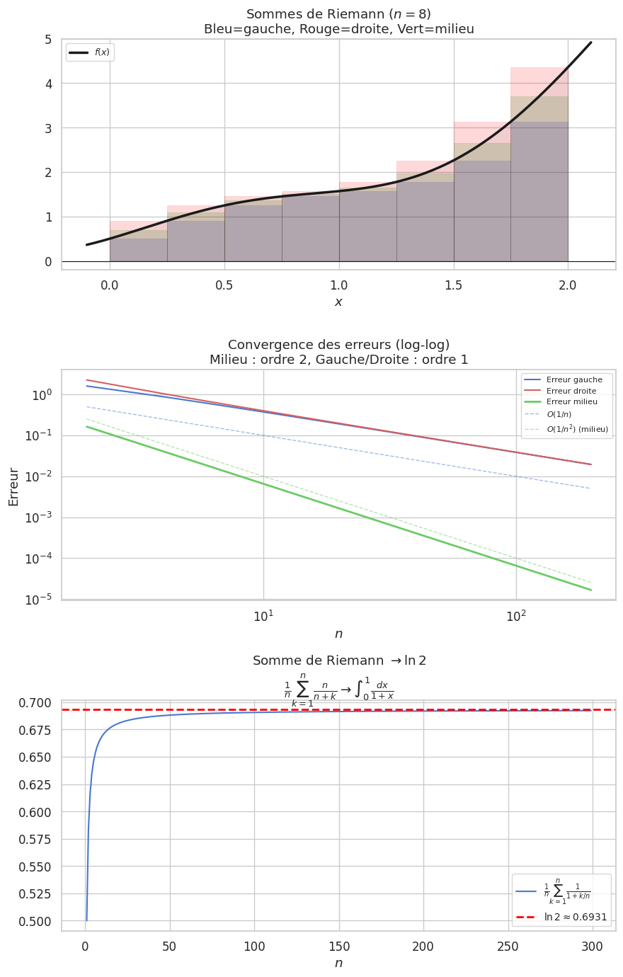
Sommes de Riemann

Proposition 186 (Approximation par sommes de Riemann)

Soit \(f\) continue sur \([a,b]\) et \((\sigma_n)\) une suite de subdivisions avec \(|\sigma_n| \to 0\). Pour tout choix de points \(\xi_i^{(n)} \in [x_{i-1}^{(n)}, x_i^{(n)}]\) :

\[\sum_{i=1}^{n} f(\xi_i^{(n)})(x_i^{(n)} - x_{i-1}^{(n)}) \xrightarrow[n \to +\infty]{} \int_a^b f(x)\,dx.\]

Exemple 62

Avec la subdivision régulière de \([0,1]\) en \(n\) intervalles et le point milieu :

\[\frac{1}{n}\sum_{k=0}^{n-1} f\!\left(\frac{k}{n}\right) \to \int_0^1 f(x)\,dx.\]

Exemples classiques :

• \(\dfrac{1}{n}\displaystyle\sum_{k=1}^{n} \dfrac{1}{1+k/n} \to \int_0^1 \dfrac{dx}{1+x} = \ln 2\)

• \(\dfrac{1}{n}\displaystyle\sum_{k=1}^{n} \sqrt{\dfrac{k}{n}} \to \int_0^1 \sqrt{x}\,dx = \dfrac{2}{3}\)

• \(\dfrac{\pi}{n}\displaystyle\sum_{k=0}^{n-1} \sin\!\left(\dfrac{k\pi}{n}\right) \to \int_0^\pi \sin x\,dx = 2\)

Show code cell source

Hide code cell source

fig, axes = plt.subplots(3, 1, figsize=(9, 14))

f = lambda x: x**2 + 0.5*np.sin(3*x) + 0.5
a_val, b_val = 0, 2
val_exacte, _ = integrate.quad(f, a_val, b_val)

# Sommes de Riemann gauche, droite, milieu
ax = axes[0]
x_fine = np.linspace(a_val - 0.1, b_val + 0.1, 500)
ax.plot(x_fine, f(x_fine), 'k-', lw=2.5, zorder=5, label='$f(x)$')

n_show = 8
dx = (b_val - a_val) / n_show
x_nodes = np.linspace(a_val, b_val - dx, n_show)

for xi, col, lbl in [(x_nodes, 'blue', 'gauche'), (x_nodes + dx, 'red', 'droite'),
                      (x_nodes + dx/2, 'green', 'milieu')]:
    for i, xpt in enumerate(x_nodes):
        h = f(xi[i])
        rect = plt.Rectangle((xpt, 0), dx, h, facecolor=col, alpha=0.15,
                               edgecolor=col, lw=0.5)
        ax.add_patch(rect)

ax.fill_between(np.linspace(a_val, b_val, 200), f(np.linspace(a_val, b_val, 200)),
                alpha=0.05, color='black')
ax.axhline(0, color='k', lw=0.8)
ax.set_title(f'Sommes de Riemann ($n={n_show}$)\nBleu=gauche, Rouge=droite, Vert=milieu')
ax.legend(fontsize=9)
ax.set_xlabel('$x$')
ax.set_ylim(-0.2, 5)

# Convergence des sommes
ax = axes[1]
n_vals = np.arange(2, 200, 2)
s_gauche, s_droite, s_milieu = [], [], []

for n in n_vals:
    dx_n = (b_val - a_val) / n
    x_g = np.linspace(a_val, b_val - dx_n, n)
    s_gauche.append(np.sum(f(x_g)) * dx_n)
    s_droite.append(np.sum(f(x_g + dx_n)) * dx_n)
    s_milieu.append(np.sum(f(x_g + dx_n/2)) * dx_n)

ax.plot(n_vals, np.abs(np.array(s_gauche) - val_exacte), 'b-', lw=1.5, label='Erreur gauche')
ax.plot(n_vals, np.abs(np.array(s_droite) - val_exacte), 'r-', lw=1.5, label='Erreur droite')
ax.plot(n_vals, np.abs(np.array(s_milieu) - val_exacte), 'g-', lw=2, label='Erreur milieu')

ax.set_xscale('log')
ax.set_yscale('log')
ax.plot(n_vals, 1/n_vals, 'b--', lw=1, alpha=0.5, label='$O(1/n)$')
ax.plot(n_vals, 1/n_vals**2, 'g--', lw=1, alpha=0.5, label='$O(1/n^2)$ (milieu)')
ax.axhline(0, color='k', lw=0.8)
ax.set_title('Convergence des erreurs (log-log)\nMilieu : ordre 2, Gauche/Droite : ordre 1')
ax.legend(fontsize=8)
ax.set_xlabel('$n$')
ax.set_ylabel('Erreur')

# Somme de Riemann classique : ln 2
ax = axes[2]
n_suite = np.arange(1, 300)
suite_ln2 = np.array([np.sum(1/(1 + np.arange(1, n+1)/n)) / n for n in n_suite])

ax.plot(n_suite, suite_ln2, 'b-', lw=1.5, label=r'$\frac{1}{n}\sum_{k=1}^n \frac{1}{1+k/n}$')
ax.axhline(np.log(2), color='red', ls='--', lw=2, label=f'$\\ln 2 \\approx {np.log(2):.4f}$')
ax.set_title('Somme de Riemann $\\to \\ln 2$\n$\\frac{1}{n}\\sum_{k=1}^n \\frac{n}{n+k} \\to \\int_0^1 \\frac{dx}{1+x}$')
ax.legend(fontsize=10)
ax.set_xlabel('$n$')

plt.tight_layout()
plt.show()

Propriétés de l’intégrale

Proposition 187 (Propriétés fondamentales)

Soient \(f, g\) intégrables sur \([a, b]\).

Linéarité : \(\displaystyle\int_a^b (\lambda f + \mu g) = \lambda\int_a^b f + \mu\int_a^b g\)

Positivité : \(f \geq 0 \Rightarrow \displaystyle\int_a^b f \geq 0\). Plus précisément, si \(f\) est continue et \(f \geq 0\) avec \(\int_a^b f = 0\), alors \(f = 0\).

Croissance : \(f \leq g \Rightarrow \displaystyle\int_a^b f \leq \int_a^b g\)

Inégalité triangulaire : \(\left|\displaystyle\int_a^b f\right| \leq \int_a^b |f|\)

Relation de Chasles : \(\displaystyle\int_a^b f = \int_a^c f + \int_c^b f\) pour \(c \in [a,b]\)

Convention : \(\displaystyle\int_b^a f = -\int_a^b f\)

Proof. Inégalité triangulaire : \(-|f| \leq f \leq |f|\), donc \(-\int_a^b |f| \leq \int_a^b f \leq \int_a^b |f|\).

\(f \geq 0\) continue et \(\int f = 0 \Rightarrow f = 0\) : Si \(f(c) > 0\), par continuité il existe \(\delta > 0\) tel que \(f > f(c)/2\) sur \([c-\delta, c+\delta] \cap [a,b]\), donc \(\int_a^b f \geq f(c)\delta > 0\). Contradiction.

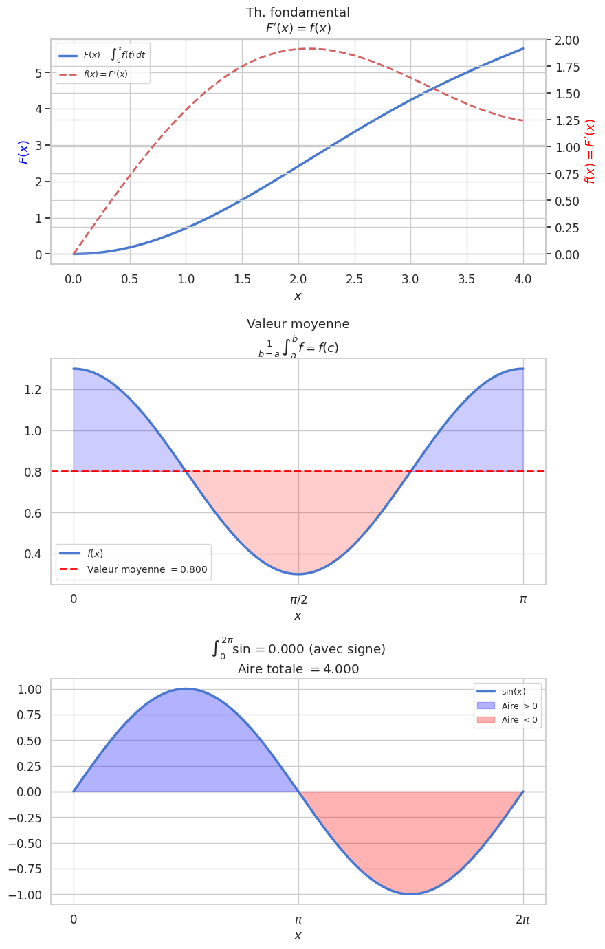
Proposition 188 (Valeur moyenne)

Soit \(f\) continue sur \([a, b]\). Il existe \(c \in [a, b]\) tel que

\[\int_a^b f(x)\,dx = f(c)(b-a).\]

La valeur \(\dfrac{1}{b-a}\displaystyle\int_a^b f\) est la valeur moyenne de \(f\) sur \([a,b]\).

Proof. Par le théorème des valeurs extrêmes, \(m \leq f \leq M\) sur \([a,b]\). Donc \(m(b-a) \leq \int_a^b f \leq M(b-a)\), soit \(m \leq \frac{1}{b-a}\int_a^b f \leq M\). Par le TVI appliqué à \(f\), il existe \(c\) tel que \(f(c) = \frac{1}{b-a}\int_a^b f\).

Théorème fondamental de l’analyse

Proposition 189 (Théorème fondamental — première forme)

Soit \(f : [a, b] \to \mathbb{R}\) continue. La fonction

\[F(x) = \int_a^x f(t)\,dt\]

est l’unique primitive de \(f\) s’annulant en \(a\) : \(F \in \mathcal{C}^1([a,b])\) et \(F' = f\).

Proof. Pour \(h \neq 0\) avec \(x + h \in [a,b]\) :

\[\frac{F(x+h) - F(x)}{h} = \frac{1}{h}\int_x^{x+h} f(t)\,dt.\]

Par le théorème de la valeur moyenne, il existe \(c_h\) entre \(x\) et \(x+h\) tel que \(\int_x^{x+h} f(t)\,dt = f(c_h) \cdot h\). Donc \(\dfrac{F(x+h)-F(x)}{h} = f(c_h) \to f(x)\) (car \(c_h \to x\) et \(f\) est continue en \(x\)).

Proposition 190 (Théorème fondamental — seconde forme (Newton-Leibniz))

Soit \(f\) continue et \(G\) une primitive quelconque de \(f\) sur \([a,b]\). Alors

\[\int_a^b f(x)\,dx = G(b) - G(a) = \Big[G(x)\Big]_a^b.\]

Proof. \(G - F\) est à dérivée nulle, donc constante. \(G(a) - F(a) = G(a)\) (car \(F(a) = 0\)). Donc \(G(b) - G(a) = F(b) - F(a) = F(b) = \int_a^b f\).

Remarque 79

Le théorème fondamental relie les deux opérations inverses que sont la dérivation et l’intégration — c’est l’un des résultats les plus profonds de l’analyse. Il a deux conséquences immédiates :

• Pour calculer \(\int_a^b f\), il suffit de trouver une primitive de \(f\).

• La dérivée de \(x \mapsto \int_a^x f(t)\,dt\) est \(f(x)\) (dérivation sous le signe \(\int\)).

Généralisation : Si \(\alpha, \beta\) sont dérivables, \(\dfrac{d}{dx}\displaystyle\int_{\alpha(x)}^{\beta(x)} f(t)\,dt = f(\beta(x))\beta'(x) - f(\alpha(x))\alpha'(x)\).

Show code cell source

Hide code cell source

fig, axes = plt.subplots(3, 1, figsize=(9, 14))

# Théorème fondamental : F(x) = int_0^x f(t) dt et F' = f
ax = axes[0]
f_tfa = lambda t: np.sin(t) + 0.5*t
x = np.linspace(0, 4, 400)
F_vals = np.array([integrate.quad(f_tfa, 0, xi)[0] for xi in x])
f_vals = f_tfa(x)

ax2 = ax.twinx()
ax.plot(x, F_vals, 'b-', lw=2.5, label='$F(x) = \\int_0^x f(t)\\,dt$')
ax2.plot(x, f_vals, 'r', lw=2, linestyle='--', label="$f(x) = F'(x)$")

ax.set_xlabel('$x$')
ax.set_ylabel('$F(x)$', color='blue')
ax2.set_ylabel("$f(x) = F'(x)$", color='red')
ax.set_title('Th. fondamental\n$F\'(x) = f(x)$')

lines1, labels1 = ax.get_legend_handles_labels()
lines2, labels2 = ax2.get_legend_handles_labels()
ax.legend(lines1 + lines2, labels1 + labels2, fontsize=9)

# Valeur moyenne
ax = axes[1]
f_moy = lambda t: np.cos(t)**2 + 0.3
a_m, b_m = 0, np.pi
x_m = np.linspace(a_m, b_m, 400)
val_moy = integrate.quad(f_moy, a_m, b_m)[0] / (b_m - a_m)

ax.plot(x_m, f_moy(x_m), 'b-', lw=2.5, label='$f(x)$')
ax.axhline(val_moy, color='red', ls='--', lw=2, label=f'Valeur moyenne $= {val_moy:.3f}$')
ax.fill_between(x_m, f_moy(x_m), val_moy, where=(f_moy(x_m) >= val_moy),
                alpha=0.2, color='blue')
ax.fill_between(x_m, f_moy(x_m), val_moy, where=(f_moy(x_m) < val_moy),
                alpha=0.2, color='red')
ax.set_title('Valeur moyenne\n$\\frac{1}{b-a}\\int_a^b f = f(c)$')
ax.legend(fontsize=10)
ax.set_xlabel('$x$')
ax.set_xticks([0, np.pi/2, np.pi])
ax.set_xticklabels(['0', '$\\pi/2$', '$\\pi$'])

# Aire géométrique (avec signe)
ax = axes[2]
f_aire = lambda t: np.sin(t)
x_a = np.linspace(0, 2*np.pi, 500)

ax.plot(x_a, f_aire(x_a), 'b-', lw=2.5, label='$\\sin(x)$')
ax.fill_between(x_a, f_aire(x_a), where=(f_aire(x_a) >= 0), alpha=0.3, color='blue', label='Aire $> 0$')
ax.fill_between(x_a, f_aire(x_a), where=(f_aire(x_a) < 0), alpha=0.3, color='red', label='Aire $< 0$')
ax.axhline(0, color='k', lw=0.8)

val_signed = integrate.quad(f_aire, 0, 2*np.pi)[0]
val_abs = integrate.quad(lambda t: np.abs(f_aire(t)), 0, 2*np.pi)[0]
ax.set_title(f'$\\int_0^{{2\\pi}} \\sin = {val_signed:.3f}$ (avec signe)\nAire totale $= {val_abs:.3f}$')
ax.legend(fontsize=9)
ax.set_xticks([0, np.pi, 2*np.pi])
ax.set_xticklabels(['0', '$\\pi$', '$2\\pi$'])
ax.set_xlabel('$x$')

plt.tight_layout()
plt.show()

Techniques d’intégration

Intégration par parties

Proposition 191 (Intégration par parties (IPP))

Soit \(u, v \in \mathcal{C}^1([a, b])\). Alors

\[\int_a^b u'(x) v(x)\,dx = \Big[u(x)v(x)\Big]_a^b - \int_a^b u(x) v'(x)\,dx.\]

Proof. \((uv)' = u'v + uv'\), donc \(u'v = (uv)' - uv'\). En intégrant sur \([a,b]\).

Remarque 80

Stratégie de choix : On choisit \(v\) facile à dériver et \(u'\) facile à intégrer. Les cas types sont :

\(u'\)	\(v\)	Résultat
\(e^{ax}\)	\(P(x)\) polynôme	Réduit le degré
\(\cos(ax)\) ou \(\sin(ax)\)	\(P(x)\)	Réduit le degré
\(e^{ax}\)	\(\sin(bx)\) ou \(\cos(bx)\)	IPP deux fois, système
\(1\)	\(\ln x\), \(\arctan x\)…	Élimine la fonction transcendante

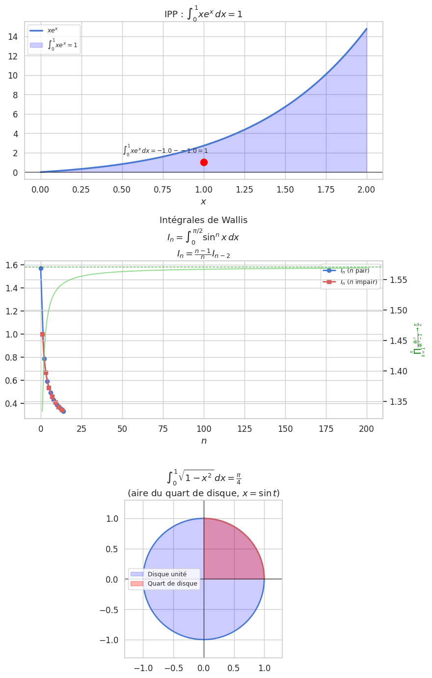
Exemple 63

1. \(\int_0^1 x e^x\,dx\) : \(u' = e^x\), \(v = x\), \(u = e^x\), \(v' = 1\).

\[\int_0^1 xe^x\,dx = \Big[xe^x\Big]_0^1 - \int_0^1 e^x\,dx = e - \Big[e^x\Big]_0^1 = e - (e-1) = 1.\]

2. \(\int_0^1 \ln x\,dx\) : \(u' = 1\), \(v = \ln x\), \(u = x\), \(v' = 1/x\).

\[\int_0^1 \ln x\,dx = \Big[x\ln x\Big]_0^1 - \int_0^1 1\,dx = (0 - 0) - 1 = -1.\]

(La limite \(x\ln x \to 0\) en \(0^+\) justifie le crochet.)

3. \(\int e^x \cos x\,dx\) : Deux IPP successives donnent un système. Posons \(I = \int e^x \cos x\,dx\). \(I = e^x \cos x + \int e^x \sin x\,dx = e^x \cos x + e^x \sin x - I\). Donc \(2I = e^x(\cos x + \sin x)\), soit \(I = \dfrac{e^x(\cos x + \sin x)}{2} + C\).

4. \(I_n = \int_0^{\pi/2} \sin^n x\,dx\) (formule de Wallis) : IPP avec \(u' = \sin x\), \(v = \sin^{n-1} x\) :

\[I_n = \Big[-\cos x \sin^{n-1} x\Big]_0^{\pi/2} + (n-1)\int_0^{\pi/2} \cos^2 x \sin^{n-2} x\,dx = (n-1)(I_{n-2} - I_n).\]

D’où la relation de récurrence de Wallis :

\[I_n = \frac{n-1}{n} I_{n-2}, \quad I_0 = \frac{\pi}{2}, \quad I_1 = 1.\]

Changement de variable

Proposition 192 (Changement de variable)

Soit \(f\) continue sur \(I\) et \(\varphi : [\alpha, \beta] \to I\) de classe \(\mathcal{C}^1\). Alors

\[\int_{\varphi(\alpha)}^{\varphi(\beta)} f(x)\,dx = \int_\alpha^\beta f(\varphi(t))\,\varphi'(t)\,dt.\]

Proof. Soit \(F\) une primitive de \(f\). Par la règle de la chaîne, \((F \circ \varphi)' = (f \circ \varphi)\varphi'\). Donc \(\int_\alpha^\beta f(\varphi(t))\varphi'(t)\,dt = \Big[F(\varphi(t))\Big]_\alpha^\beta = F(\varphi(\beta)) - F(\varphi(\alpha)) = \int_{\varphi(\alpha)}^{\varphi(\beta)} f(x)\,dx\).

Exemple 64

1. \(\int_0^1 \frac{dx}{\sqrt{1-x^2}}\) : \(x = \sin t\), \(dx = \cos t\,dt\), \(1-x^2 = \cos^2 t\).

\[\int_0^{\pi/2} \frac{\cos t\,dt}{\cos t} = \frac{\pi}{2}.\]

2. \(\int_0^1 \sqrt{1-x^2}\,dx\) : \(x = \sin t\), \(dx = \cos t\,dt\).

\[\int_0^{\pi/2} \cos^2 t\,dt = \frac{1}{2}\int_0^{\pi/2}(1+\cos 2t)\,dt = \frac{\pi}{4}.\]

C’est l’aire du quart de disque unité, cohérent avec \(\pi r^2/4 = \pi/4\).

3. \(\int_0^{+\infty} e^{-x^2}\,dx\) : \(t = \sqrt{x}\), \(x = t^2\), \(dx = 2t\,dt\).

\[\int_0^{+\infty} e^{-t^2} \cdot 2t\,\frac{dt}{2\sqrt{t^2}} = \ldots\]

On verra ci-dessous (Gauss) que ce résultat nécessite une autre approche.

4. Substitution \(t = \tan(\theta/2)\) : Pour les intégrales de fractions rationnelles en \(\cos\theta, \sin\theta\) :

\[\cos\theta = \frac{1-t^2}{1+t^2}, \quad \sin\theta = \frac{2t}{1+t^2}, \quad d\theta = \frac{2\,dt}{1+t^2}.\]

\[\int_0^{\pi/2}\frac{d\theta}{2+\cos\theta} = \int_0^1 \frac{1}{2 + \frac{1-t^2}{1+t^2}} \cdot \frac{2\,dt}{1+t^2} = \int_0^1 \frac{2\,dt}{3+t^2} = \frac{2}{\sqrt{3}}\arctan\!\frac{1}{\sqrt{3}} = \frac{\pi}{3\sqrt{3}}.\]

Primitives des fractions rationnelles

Proposition 193 (Méthode de décomposition en éléments simples)

Toute fraction rationnelle \(R(x) = P(x)/Q(x)\) (avec \(\deg P < \deg Q\) après division euclidienne) se décompose sur \(\mathbb{R}\) en éléments simples :

\[R(x) = \sum_{\text{racines réelles } a_i} \sum_{k=1}^{m_i} \frac{A_{i,k}}{(x-a_i)^k} + \sum_{\text{facteurs } x^2+p_j x+q_j} \sum_{k=1}^{n_j} \frac{B_{j,k} x + C_{j,k}}{(x^2+p_j x+q_j)^k}.\]

Remarque 81

Primitives des éléments simples :

Élément simple	Primitive
\(\dfrac{A}{x-a}\)	$A\ln
\(\dfrac{A}{(x-a)^k}\) (\(k \geq 2\))	\(\dfrac{A}{(1-k)(x-a)^{k-1}}\)
\(\dfrac{Bx+C}{x^2+px+q}\)	\(\dfrac{B}{2}\ln(x^2+px+q) + \dfrac{C - Bp/2}{\sqrt{q-p^2/4}}\arctan\!\dfrac{x+p/2}{\sqrt{q-p^2/4}}\)

Exemple 65

1. \(\int \frac{dx}{x^2-1} = \int \frac{1}{2}\left(\frac{1}{x-1} - \frac{1}{x+1}\right)dx = \frac{1}{2}\ln\left|\frac{x-1}{x+1}\right| + C\).

2. \(\int \frac{x+2}{x^2+2x+5}\,dx\) : \(x^2+2x+5 = (x+1)^2 + 4\).

\[\int \frac{x+2}{(x+1)^2+4}\,dx = \int \frac{(x+1)+1}{(x+1)^2+4}\,dx = \frac{1}{2}\ln(x^2+2x+5) + \frac{1}{2}\arctan\!\frac{x+1}{2} + C.\]

3. \(\int_0^1 \frac{dx}{(1+x^2)^2}\) : On pose \(x = \tan\theta\), \(dx = d\theta/\cos^2\theta\), \(1+x^2 = 1/\cos^2\theta\).

\[\int_0^{\pi/4} \cos^2\theta\,d\theta = \int_0^{\pi/4}\frac{1+\cos 2\theta}{2}\,d\theta = \frac{\pi}{8} + \frac{1}{4}.\]

4. Décomposition en éléments simples avec racine multiple :

\[\frac{1}{x^2(x+1)} = \frac{A}{x} + \frac{B}{x^2} + \frac{C}{x+1}.\]

En multipliant par \(x^2\) et évaluant en 0 : \(B = 1\). En multipliant par \(x+1\) et évaluant en \(-1\) : \(C = 1\). En regardant le comportement en \(+\infty\) (\(\sim A/x\)) ou par identification : \(A = -1\).

\[\int \frac{dx}{x^2(x+1)} = -\ln|x| - \frac{1}{x} + \ln|x+1| + C.\]

Show code cell source

Hide code cell source

fig, axes = plt.subplots(3, 1, figsize=(9, 14))

# IPP : int x e^x et visualisation
ax = axes[0]
x = np.linspace(0, 2, 400)
f_ipp = x * np.exp(x)
F_ipp = (x - 1) * np.exp(x)  # primitive exacte

ax.plot(x, f_ipp, 'b-', lw=2.5, label='$xe^x$')
ax.fill_between(x, f_ipp, alpha=0.2, color='blue', label=f'$\\int_0^1 xe^x = 1$')
ax.scatter([1], [1], color='red', s=100, zorder=5)
ax.annotate(f'$\\int_0^1 xe^x\\,dx = {(0-1)*np.exp(0):.1f} - {(0-1)*1:.1f} = 1$',
            xy=(0.5, 2), fontsize=9)
ax.axhline(0, color='k', lw=0.8)
ax.set_title('IPP : $\\int_0^1 xe^x\\,dx = 1$')
ax.legend(fontsize=9)
ax.set_xlabel('$x$')

# Wallis
ax = axes[1]
def I_wallis(n):
    if n == 0: return np.pi/2
    if n == 1: return 1.0
    return (n-1)/n * I_wallis(n-2)

ns = np.arange(0, 15)
I_vals = np.array([I_wallis(n) for n in ns])

ax.plot(ns[::2], I_vals[::2], 'bo-', lw=2, ms=6, label='$I_n$ ($n$ pair)')
ax.plot(ns[1::2], I_vals[1::2], 'rs-', lw=2, ms=6, label='$I_n$ ($n$ impair)')
ax.set_title('Intégrales de Wallis\n$I_n = \\int_0^{\\pi/2} \\sin^n x\\,dx$\n$I_n = \\frac{n-1}{n}I_{n-2}$')
ax.legend(fontsize=9)
ax.set_xlabel('$n$')

# Produit de Wallis
n_max = 200
W_partial = np.cumprod([(4*k**2)/(4*k**2 - 1) for k in range(1, n_max+1)])
ax2 = ax.twinx()
ax2.plot(range(1, n_max+1), W_partial, 'g-', lw=1.5, alpha=0.7)
ax2.axhline(np.pi/2, color='green', ls='--', lw=1, alpha=0.7)
ax2.set_ylabel('$\\prod_{k=1}^n \\frac{4k^2}{4k^2-1} \\to \\frac{\\pi}{2}$', color='green', fontsize=8)

# Changement de variable : aire du disque
ax = axes[2]
theta = np.linspace(0, 2*np.pi, 400)
ax.fill(np.cos(theta), np.sin(theta), alpha=0.2, color='blue', label='Disque unité')
ax.plot(np.cos(theta), np.sin(theta), 'b-', lw=2)

# Visualiser le changement x = sin(t)
t_arr = np.linspace(0, np.pi/2, 400)
x_arr = np.sin(t_arr)
y_arr = np.sqrt(1 - x_arr**2)

ax.fill_between(x_arr, y_arr, alpha=0.3, color='red', label='Quart de disque')
ax.plot(x_arr, y_arr, 'r-', lw=2)
ax.axhline(0, color='k', lw=0.8)
ax.axvline(0, color='k', lw=0.8)
ax.set_aspect('equal')
ax.set_xlim(-1.3, 1.3)
ax.set_ylim(-1.3, 1.3)
ax.set_title('$\\int_0^1 \\sqrt{1-x^2}\\,dx = \\frac{\\pi}{4}$\n(aire du quart de disque, $x=\\sin t$)')
ax.legend(fontsize=9)

plt.tight_layout()
plt.show()

Intégration des fonctions trigonométriques

Remarque 82

Les intégrales de fonctions trigonométriques se réduisent aux cas suivants :

Puissances de \(\sin\) et \(\cos\) :

• \(\sin^n x\) ou \(\cos^n x\) : linéarisation par les formules d’Euler ou les formules de duplication.

• \(\sin^p x \cos^q x\) : si \(p\) ou \(q\) est impair, substitution \(u = \cos x\) ou \(u = \sin x\).

Formes rationnelles en \(\sin x\), \(\cos x\) :

• Substitution \(t = \tan(x/2)\) (méthode universelle, mais souvent lourde).

• Reconnaissance directe si \(f\) est de la forme \(\frac{\cos x}{\sin^k x}\) (substitution \(u = \sin x\)).

\(\sin(ax)\sin(bx)\), etc. : Formules produit-somme, puis intégration directe.

Exemple 66

\(\int \sin^4 x\,dx\) : Linéarisation. \(\sin^4 x = \left(\frac{1-\cos 2x}{2}\right)^2 = \frac{1 - 2\cos 2x + \cos^2 2x}{4} = \frac{3/2 - 2\cos 2x + \cos 4x/2}{4}.\)

\[\int \sin^4 x\,dx = \frac{3x}{8} - \frac{\sin 2x}{4} + \frac{\sin 4x}{32} + C.\]

\(\int \frac{dx}{2 + \sin x}\) : Substitution \(t = \tan(x/2)\). \(2 + \sin x = 2 + \frac{2t}{1+t^2} = \frac{2(1+t^2)+2t}{1+t^2}\), \(dx = \frac{2\,dt}{1+t^2}\).

\[\int \frac{2\,dt}{2t^2+2t+2} = \int \frac{dt}{t^2+t+1} = \int \frac{dt}{(t+1/2)^2 + 3/4} = \frac{2}{\sqrt{3}}\arctan\!\frac{2t+1}{\sqrt{3}} + C.\]

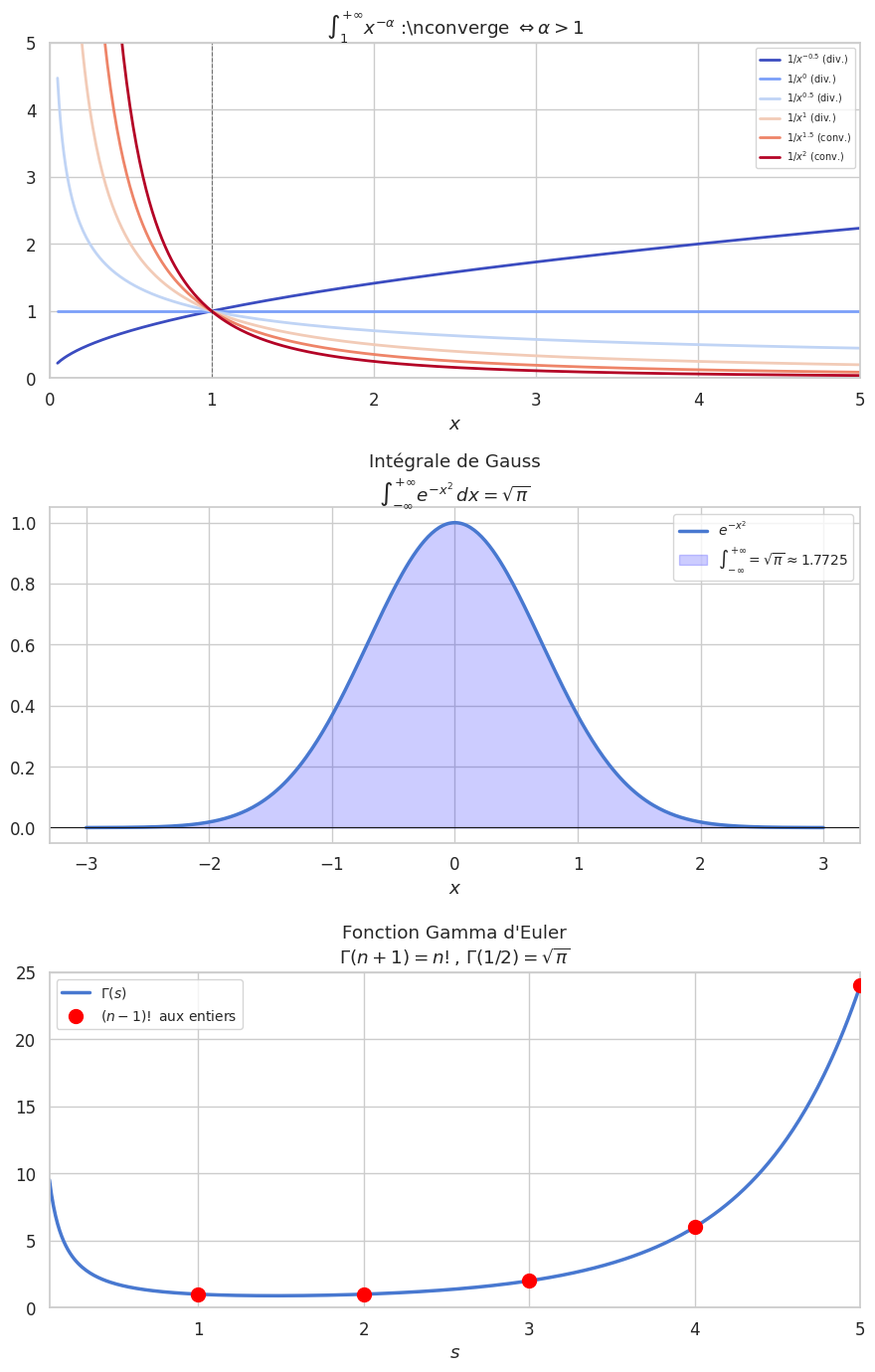
Intégrales généralisées (impropres)

Définition 127 (Intégrale impropre)

Soit \(f : [a, b[ \to \mathbb{R}\) continue (avec \(b \in \mathbb{R}\) ou \(b = +\infty\), ou \(f\) non bornée en \(b\)). L”intégrale impropre converge si \(\lim_{t \to b^-} \int_a^t f(x)\,dx\) est finie. On la note \(\int_a^b f(x)\,dx\).

De même en \(a^+\) si \(f\) est définie sur \(]a, b]\).

Exemple 67

Convergentes :

• \(\int_1^{+\infty} \frac{dx}{x^2} = \lim_{t \to +\infty}\left[-\frac{1}{x}\right]_1^t = 1\).

• \(\int_0^1 \frac{dx}{\sqrt{x}} = \lim_{t \to 0^+} [2\sqrt{x}]_t^1 = 2\) (malgré \(f(x) \to +\infty\) en 0).

• \(\int_0^{+\infty} e^{-x}\,dx = 1\).

Divergentes :

• \(\int_1^{+\infty} \frac{dx}{x} = +\infty\).

• \(\int_0^1 \frac{dx}{x} = +\infty\) (singularité non intégrable).

Proposition 194 (Intégrales de Riemann généralisées)

\[\int_1^{+\infty} \frac{dx}{x^\alpha} \text{ converge} \iff \alpha > 1. \quad \left(\text{valeur} = \frac{1}{\alpha-1}\right)\]

\[\int_0^1 \frac{dx}{x^\alpha} \text{ converge} \iff \alpha < 1. \quad \left(\text{valeur} = \frac{1}{1-\alpha}\right)\]

\[\int_0^{+\infty} e^{-\lambda x}\,dx = \frac{1}{\lambda} \quad (\lambda > 0).\]

Proof. Pour \(\alpha \neq 1\) : \(\int_1^t \frac{dx}{x^\alpha} = \frac{t^{1-\alpha}-1}{1-\alpha}.\) Si \(\alpha > 1\) : \(t^{1-\alpha} = t^{-(α-1)} \to 0\), donc la limite vaut \(\frac{1}{\alpha-1}\). Si \(\alpha < 1\) : \(t^{1-\alpha} \to +\infty\). Si \(\alpha = 1\) : \(\int_1^t \frac{dx}{x} = \ln t \to +\infty\).

Critères de convergence

Proposition 195 (Critère de comparaison)

Soient \(0 \leq f(x) \leq g(x)\) sur \([a, +\infty[\).

• \(\int_a^{+\infty} g\) converge \(\Rightarrow\) \(\int_a^{+\infty} f\) converge.

• \(\int_a^{+\infty} f\) diverge \(\Rightarrow\) \(\int_a^{+\infty} g\) diverge.

Proposition 196 (Critère de comparaison par équivalents)

Si \(f, g > 0\) et \(f \sim g\) en \(b\) (borne d’intégration), alors \(\int f\) et \(\int g\) ont même nature.

Proposition 197 (Convergence absolue)

Si \(\int_a^b |f(x)|\,dx\) converge, alors \(\int_a^b f(x)\,dx\) converge et

\[\left|\int_a^b f(x)\,dx\right| \leq \int_a^b |f(x)|\,dx.\]

La réciproque est fausse : l’intégrale peut converger sans converger absolument.

Exemple 68

\(\int_1^{+\infty} \frac{\sin x}{x}\,dx\) converge (par IPP : \(\int_1^t \frac{\sin x}{x}\,dx = \left[-\frac{\cos x}{x}\right]_1^t - \int_1^t \frac{\cos x}{x^2}\,dx\), les deux termes convergent).

Mais \(\int_1^{+\infty} \frac{|\sin x|}{x}\,dx\) diverge (par comparaison : \(|\sin x|/x \geq \frac{1}{2(k+1)\pi}\) sur \([k\pi, (k+1)\pi]\), et \(\sum 1/k\) diverge).

Intégrale de Gauss et fonctions classiques

Proposition 198 (Intégrale de Gauss)

\[\int_{-\infty}^{+\infty} e^{-x^2}\,dx = \sqrt{\pi}.\]

Proof. Calcul par passage en polaires. Posons \(I = \int_0^{+\infty} e^{-x^2}\,dx > 0\).

\[I^2 = \int_0^{+\infty}\int_0^{+\infty} e^{-(x^2+y^2)}\,dx\,dy.\]

En coordonnées polaires (\(x = r\cos\theta\), \(y = r\sin\theta\), jacobien \(r\)) sur le premier quadrant (\(\theta \in [0, \pi/2]\), \(r \geq 0\)) :

\[I^2 = \int_0^{\pi/2}\int_0^{+\infty} e^{-r^2} r\,dr\,d\theta = \frac{\pi}{2} \cdot \frac{1}{2} = \frac{\pi}{4}.\]

Donc \(I = \sqrt{\pi}/2\) et \(\int_{-\infty}^{+\infty} e^{-x^2}\,dx = 2I = \sqrt{\pi}\).

Définition 128 (Fonction Gamma d’Euler)

\[\Gamma(s) = \int_0^{+\infty} t^{s-1} e^{-t}\,dt, \quad s > 0.\]

Proposition 199 (Propriétés de \(\Gamma\))

• \(\Gamma(n+1) = n!\) pour \(n \in \mathbb{N}\) (la fonction Gamma étend la factorielle)

• \(\Gamma(s+1) = s\,\Gamma(s)\) (relation fonctionnelle, par IPP)

• \(\Gamma(1/2) = \sqrt{\pi}\) (lien avec l’intégrale de Gauss)

• \(\Gamma\) est log-convexe et \(\mathcal{C}^\infty\) sur \(]0, +\infty[\)

Proof. Relation \(\Gamma(s+1) = s\Gamma(s)\) : Par IPP avec \(u = t^s\) et \(v' = e^{-t}\) :

\[\Gamma(s+1) = \Big[-t^s e^{-t}\Big]_0^{+\infty} + s\int_0^{+\infty} t^{s-1} e^{-t}\,dt = s\Gamma(s).\]

\(\Gamma(1/2) = \sqrt{\pi}\) : \(\Gamma(1/2) = \int_0^{+\infty} t^{-1/2} e^{-t}\,dt\). Poser \(t = u^2\) : \(= 2\int_0^{+\infty} e^{-u^2}\,du = \sqrt{\pi}\).

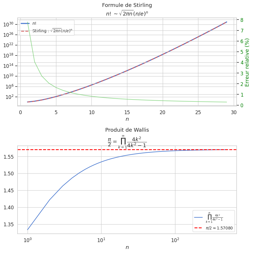
Proposition 200 (Formule de Stirling)

\[n! \sim \sqrt{2\pi n}\left(\frac{n}{e}\right)^n \quad (n \to +\infty).\]

Plus précisément : \(n! = \sqrt{2\pi n}\left(\frac{n}{e}\right)^n e^{\theta_n/(12n)}\) avec \(\theta_n \in ]0,1[\).

Show code cell source

Hide code cell source

fig, axes = plt.subplots(3, 1, figsize=(9, 14))

# Intégrales impropres : convergence vs divergence
ax = axes[0]
x = np.linspace(0.05, 5, 500)

alphas = [-0.5, 0, 0.5, 1, 1.5, 2]
colors = plt.cm.coolwarm(np.linspace(0, 1, len(alphas)))

for alpha, col in zip(alphas, colors):
    ax.plot(x, x**(-alpha), color=col, lw=2,
            label=f'$1/x^{{{alpha}}}$ ({"conv." if alpha > 1 else "div."})')

ax.axhline(0, color='k', lw=0.8)
ax.axvline(1, color='k', ls='--', lw=0.8, alpha=0.5)
ax.set_ylim(0, 5)
ax.set_xlim(0, 5)
ax.set_title(r'$\int_1^{+\infty} x^{-\alpha}$ :\nconverge $\Leftrightarrow \alpha > 1$')
ax.legend(fontsize=7)
ax.set_xlabel('$x$')

# Gauss : approximations de sqrt(pi)/2
ax = axes[1]
n_gauss = np.arange(1, 300)
I_gauss = np.array([integrate.quad(lambda t: np.exp(-t**2), 0, R)[0] for R in [1, 2, 3, 5, 10]])

x_g = np.linspace(-3, 3, 400)
ax.plot(x_g, np.exp(-x_g**2), 'b-', lw=2.5, label='$e^{-x^2}$')
ax.fill_between(x_g, np.exp(-x_g**2), alpha=0.2, color='blue',
                label=f'$\\int_{{-\\infty}}^{{+\\infty}} = \\sqrt{{\\pi}} \\approx {np.sqrt(np.pi):.4f}$')
ax.axhline(0, color='k', lw=0.8)
ax.set_title(f'Intégrale de Gauss\n$\\int_{{-\\infty}}^{{+\\infty}} e^{{-x^2}}\\,dx = \\sqrt{{\\pi}}$')
ax.legend(fontsize=10)
ax.set_xlabel('$x$')

# Fonction Gamma et comparaison avec (n-1)!
ax = axes[2]
s_vals = np.linspace(0.1, 5, 400)
gamma_vals = np.array([integrate.quad(lambda t: t**(s-1)*np.exp(-t), 0, np.inf)[0]
                        for s in s_vals])

ax.plot(s_vals, gamma_vals, 'b-', lw=2.5, label='$\\Gamma(s)$')
n_vals_g = np.arange(1, 6)
ax.scatter(n_vals_g, [math.factorial(n-1) for n in n_vals_g],
           color='red', s=100, zorder=5, label='$(n-1)!$ aux entiers')

ax.set_ylim(0, 25)
ax.set_xlim(0.1, 5)
ax.set_title('Fonction Gamma d\'Euler\n$\\Gamma(n+1) = n!$, $\\Gamma(1/2)=\\sqrt{\\pi}$')
ax.legend(fontsize=10)
ax.set_xlabel('$s$')
ax.axhline(0, color='k', lw=0.8)

plt.tight_layout()
plt.show()

Show code cell source

Hide code cell source

# Stirling et formule de Wallis
fig, axes = plt.subplots(2, 1, figsize=(9, 9))

# Stirling
ax = axes[0]
n_stir = np.arange(1, 30)
fact_exact = np.array([math.factorial(n) for n in n_stir], dtype=float)
stirling = np.sqrt(2*np.pi*n_stir) * (n_stir/np.e)**n_stir

ax.semilogy(n_stir, fact_exact, 'b-', lw=2.5, label='$n!$')
ax.semilogy(n_stir, stirling, 'r--', lw=2, label="Stirling : $\\sqrt{2\\pi n}(n/e)^n$")
ax.set_title('Formule de Stirling\n$n! \\sim \\sqrt{2\\pi n}(n/e)^n$')
ax.legend(fontsize=10)
ax.set_xlabel('$n$')

# Erreur relative de Stirling
ax2 = ax.twinx()
err_rel = np.abs(fact_exact - stirling) / fact_exact * 100
ax2.plot(n_stir, err_rel, 'g-', lw=1.5, alpha=0.7)
ax2.set_ylabel('Erreur relative (%)', color='green')
ax2.tick_params(axis='y', labelcolor='green')

# Produit de Wallis : π/2 = ∏ (4k²)/(4k²-1)
ax = axes[1]
N_max = 500
k_arr = np.arange(1, N_max+1)
wallis_partial = np.cumprod(4*k_arr**2 / (4*k_arr**2 - 1))

ax.plot(k_arr, wallis_partial, 'b-', lw=1.5, label='$\\prod_{k=1}^n \\frac{4k^2}{4k^2-1}$')
ax.axhline(np.pi/2, color='red', ls='--', lw=2, label=f'$\\pi/2 \\approx {np.pi/2:.5f}$')
ax.set_xscale('log')
ax.set_title('Produit de Wallis\n$\\dfrac{\\pi}{2} = \\prod_{k=1}^\\infty \\dfrac{4k^2}{4k^2-1}$')
ax.legend(fontsize=10)
ax.set_xlabel('$n$')

print(f"Wallis (n=500): {wallis_partial[-1]:.6f}, π/2 = {np.pi/2:.6f}")
print(f"Stirling (n=20): erreur relative = {err_rel[19]:.4f}%")

plt.tight_layout()
plt.show()

Wallis (n=500): 1.570012, π/2 = 1.570796
Stirling (n=20): erreur relative = 0.4158%

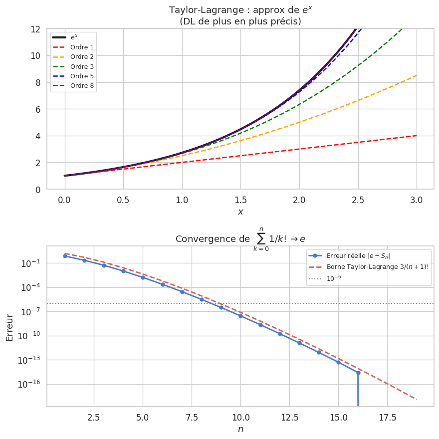
Formule de Taylor avec reste intégral

Proposition 201 (Reste intégral (rappel et application))

Pour \(f \in \mathcal{C}^{n+1}\) :

\[f(x) = \sum_{k=0}^n \frac{f^{(k)}(a)}{k!}(x-a)^k + \underbrace{\int_a^x \frac{(x-t)^n}{n!}f^{(n+1)}(t)\,dt}_{R_n(x)}.\]

Encadrement de l’erreur : Si \(|f^{(n+1)}| \leq M\) sur \([a, x]\) :

\[|R_n(x)| \leq M\frac{|x-a|^{n+1}}{(n+1)!}.\]

Reste de Lagrange : Il existe \(c\) entre \(a\) et \(x\) tel que \(R_n(x) = \dfrac{f^{(n+1)}(c)}{(n+1)!}(x-a)^{n+1}\).

Exemple 69

Calcul de \(e\) à \(10^{-6}\) près : \(e^1 = \sum_{k=0}^n \frac{1}{k!} + R_n\) avec \(|R_n| \leq \frac{e}{(n+1)!} \leq \frac{3}{(n+1)!}\). \(\frac{3}{(n+1)!} < 10^{-6}\) si \((n+1)! > 3 \times 10^6\), soit \(n \geq 9\) (\(10! = 3628800\)). Vérification numérique :

\[e \approx \sum_{k=0}^{9} \frac{1}{k!} = 1 + 1 + \frac{1}{2} + \frac{1}{6} + \frac{1}{24} + \cdots \approx 2.7182818.\]

Show code cell source

Hide code cell source

fig, axes = plt.subplots(2, 1, figsize=(9, 9))

# Reste intégral pour e^x
ax = axes[0]
x_arr = np.linspace(0, 3, 400)

ax.plot(x_arr, np.exp(x_arr), 'k-', lw=3, label='$e^x$')

for n, col in [(1, 'red'), (2, 'orange'), (3, 'green'), (5, 'blue'), (8, 'purple')]:
    approx = sum(x_arr**k / math.factorial(k) for k in range(n+1))
    reste = np.abs(np.exp(x_arr) - approx)
    borne = np.exp(x_arr) * x_arr**(n+1) / math.factorial(n+1)  # borne de Taylor-Lagrange
    ax.plot(x_arr, approx, '--', color=col, lw=1.8, label=f'Ordre {n}')

ax.set_ylim(0, 12)
ax.set_title('Taylor-Lagrange : approx de $e^x$\n(DL de plus en plus précis)')
ax.legend(fontsize=9)
ax.set_xlabel('$x$')

# Approximation de e : convergence
ax = axes[1]
n_terms = np.arange(1, 20)
e_approx = np.array([sum(1/math.factorial(k) for k in range(n+1)) for n in n_terms])
erreur = np.abs(e_approx - np.e)
borne_th = np.array([3/math.factorial(n+1) for n in n_terms])

ax.semilogy(n_terms, erreur, 'b-o', lw=2, ms=5, label='Erreur réelle $|e - S_n|$')
ax.semilogy(n_terms, borne_th, 'r--', lw=2, label='Borne Taylor-Lagrange $3/(n+1)!$')
ax.axhline(1e-6, color='gray', ls=':', lw=1.5, label='$10^{-6}$')
ax.set_title('Convergence de $\\sum_{k=0}^n 1/k! \\to e$')
ax.legend(fontsize=9)
ax.set_xlabel('$n$')
ax.set_ylabel('Erreur')

plt.tight_layout()
plt.show()

Intégrales dépendant d’un paramètre

Proposition 202 (Continuité sous le signe intégral)

Soit \(f : [a,b] \times [c,d] \to \mathbb{R}\) continue. Alors

\[F(\lambda) = \int_a^b f(x, \lambda)\,dx\]

est continue sur \([c,d]\).

Proposition 203 (Dérivation sous le signe intégral)

Soit \(f\) continue sur \([a,b] \times [c,d]\) et \(\partial_\lambda f\) continue sur \([a,b] \times [c,d]\). Alors \(F\) est \(\mathcal{C}^1\) sur \([c,d]\) et

\[F'(\lambda) = \int_a^b \frac{\partial f}{\partial \lambda}(x, \lambda)\,dx.\]

Remarque 83

Ces résultats s’étendent aux intégrales impropres sous des conditions de domination (théorème de convergence dominée de Lebesgue, hors programme). Le cas compact est le plus utilisé en pratique.

Exemple 70

Calcul de \(\int_0^1 x^n\ln x\,dx\) par dérivation sous le signe \(\int\). Posons

\[F(\lambda) = \int_0^1 x^\lambda\,dx = \frac{1}{\lambda+1} \quad (\lambda > -1).\]

En dérivant par rapport à \(\lambda\) :

\[F'(\lambda) = \int_0^1 x^\lambda \ln x\,dx = -\frac{1}{(\lambda+1)^2}.\]

En \(\lambda = n\) : \(\displaystyle\int_0^1 x^n \ln x\,dx = -\frac{1}{(n+1)^2}\).