Séries entières

Il n’y a pas de problème résolu, il n’y a que des problèmes plus ou moins résolus.

Henri Poincaré

Introduction

Les séries entières \(\sum a_n z^n\) sont des séries de fonctions polynomiales, convergentes sur un disque ouvert dont le rayon est déterminé par les coefficients. Elles généralisent les polynômes à l’infini et constituent l’outil fondamental pour représenter les fonctions analytiques. Leur régularité (dérivation et intégration terme à terme) est remarquable.

Show code cell source

Hide code cell source

import numpy as np
import matplotlib.pyplot as plt
import math

fig, axes = plt.subplots(3, 1, figsize=(9, 14))

# --- Rayon de convergence : trois cas ---
ax = axes[0]
x = np.linspace(-1.8, 1.8, 500)
x_safe = np.where(np.abs(x) < 0.999, x, np.nan)

# Série géométrique : R=1
partial_geo = {N: np.sum([x_safe**k for k in range(N+1)], axis=0) for N in [3, 7, 15]}
colors_geo = plt.cm.Blues(np.linspace(0.4, 0.9, 3))
for (N, s), c in zip(partial_geo.items(), colors_geo):
    ax.plot(x, s, color=c, lw=1.5, alpha=0.8, label=f'$S_{N}$ (géom.)')

with np.errstate(divide='ignore', invalid='ignore'):
    geo_exact = np.where(np.abs(x) < 1, 1/(1-x), np.nan)
ax.plot(x, geo_exact, 'b--', lw=2.5, label='$1/(1-x)$')
ax.axvline(-1, color='red', lw=1.5, linestyle=':', alpha=0.7)
ax.axvline(1, color='red', lw=1.5, linestyle=':', label='$R=1$')
ax.set_xlim(-1.8, 1.8); ax.set_ylim(-4, 6)
ax.set_title('$\\sum x^n = 1/(1-x)$\nrayon $R=1$', fontsize=10)
ax.set_xlabel('$x$'); ax.legend(fontsize=7)

# --- Disque de convergence dans le plan complexe ---
ax = axes[1]
theta = np.linspace(0, 2*np.pi, 300)
# R=1
circle1 = plt.Circle((0,0), 1, fill=True, facecolor='lightblue', edgecolor='blue', lw=2, alpha=0.4)
ax.add_patch(circle1)
ax.text(0, 0, 'CV absolue\n$|z| < R$', ha='center', va='center', fontsize=9)

# R=2 (exemple)
circle2 = plt.Circle((0,0), 2, fill=False, edgecolor='green', lw=2, linestyle='--')
ax.add_patch(circle2)
ax.text(1.5, 0.2, '$|z|=R$\n?', fontsize=8, color='green')

# R=3 (diverge)
circle3 = plt.Circle((0,0), 3, fill=False, edgecolor='red', lw=1, linestyle=':')
ax.add_patch(circle3)
ax.text(2.5, 0, 'Div.\n$|z|>R$', fontsize=8, color='red')

ax.axhline(0, color='k', lw=0.5); ax.axvline(0, color='k', lw=0.5)
ax.set_xlim(-3.5, 3.5); ax.set_ylim(-3.5, 3.5)
ax.set_aspect('equal')
ax.set_title('Disque de convergence dans $\\mathbb{C}$\n$R$ = rayon de convergence', fontsize=10)
ax.set_xlabel('Re'); ax.set_ylabel('Im')

# --- DSE classiques : convergence vers la cible ---
ax = axes[2]
x3 = np.linspace(-2, 2, 500)

# ln(1+x) = sum (-1)^(n-1) x^n / n, R=1
x_ln = np.linspace(-0.99, 0.99, 300)
ax.plot(x_ln, np.log(1+x_ln), 'k-', lw=3, label='$\\ln(1+x)$')
for N, c in zip([3, 7, 15], plt.cm.Oranges(np.linspace(0.4, 0.9, 3))):
    s = sum((-1)**(n-1) * x_ln**n / n for n in range(1, N+1))
    ax.plot(x_ln, s, color=c, lw=1.8, label=f'$S_{N}$')

ax.set_xlim(-1.1, 1.1); ax.set_ylim(-2, 1)
ax.axvline(-1, color='red', lw=1, linestyle=':', alpha=0.5)
ax.axvline(1, color='red', lw=1, linestyle=':', alpha=0.5)
ax.set_title('$\\ln(1+x) = \\sum \\frac{(-1)^{n-1}}{n}x^n$\n$R=1$', fontsize=10)
ax.set_xlabel('$x$'); ax.legend(fontsize=7)

plt.suptitle('Séries entières : rayon de convergence et DSE classiques', fontsize=13, fontweight='bold')
plt.tight_layout()
plt.show()

Rayon de convergence

Définition 217 (Série entière)

Une série entière est \(\sum_{n=0}^\infty a_n z^n\) où \((a_n) \subset \mathbb{C}\) et \(z \in \mathbb{C}\) (ou \(\mathbb{R}\)).

Lemme 1 (Lemme d’Abel)

Si \((a_n z_0^n)\) est bornée (par \(M > 0\)), alors \(\sum a_n z^n\) converge absolument pour tout \(|z| < |z_0|\).

Proof. Pour \(|z| < |z_0|\), posons \(r = |z|/|z_0| < 1\). \(|a_n z^n| = |a_n z_0^n| \cdot |z/z_0|^n \leq M r^n\). La série \(\sum Mr^n\) est une série géométrique convergente.

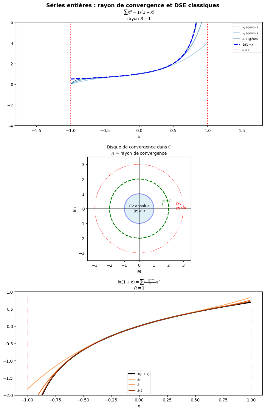
Théorème 24 (Rayon de convergence — Formule de Hadamard)

Il existe \(R \in [0, +\infty]\) tel que :

• \(|z| < R\) : convergence absolue

• \(|z| > R\) : divergence grossière (\(a_n z^n \not\to 0\))

• \(|z| = R\) : aucune conclusion générale

Formule de Hadamard : \(\dfrac{1}{R} = \limsup_{n \to +\infty} |a_n|^{1/n}\)

Proof. Posons \(L = \limsup |a_n|^{1/n}\), \(R = 1/L\).

\(|z| < R\) : \(|z|L < 1\). Choisir \(r \in (|z|L, 1)\). Pour \(n\) assez grand, \(|a_n|^{1/n} < r/|z|\), donc \(|a_n z^n| < r^n\) — série convergente.

\(|z| > R\) : \(|z|L > 1\). Pour une infinité de \(n\), \(|a_n|^{1/n} > 1/|z|\), donc \(|a_n z^n| > 1\) infiniment souvent : la série diverge grossièrement.

Proposition 294 (Règle de d’Alembert)

Si \(a_n \neq 0\) et \(|a_{n+1}/a_n| \to L\), alors \(R = 1/L\).

Exemple 107

Série	Coefficients	\(R\)	Comportement en \(\pm R\)
\(\sum x^n\)	\(a_n = 1\)	\(1\)	diverge aux deux bords
\(\sum x^n/n\)	\(a_n = 1/n\)	\(1\)	CV en \(-1\) (Leibniz), div. en \(1\)
\(\sum x^n/n^2\)	\(a_n = 1/n^2\)	\(1\)	CV en \(\pm 1\)
\(\sum x^n/n!\)	\(a_n = 1/n!\)	\(+\infty\)	\(e^x\)
\(\sum n! x^n\)	\(a_n = n!\)	\(0\)	trivial

Propriétés analytiques

Théorème 25 (Convergence normale sur les compacts)

Pour tout \(r < R\), la série \(\sum a_n z^n\) converge normalement sur \(\overline{D}(0, r)\) :

\[\sum_{n \geq 0} \sup_{|z| \leq r} |a_n z^n| = \sum_{n \geq 0} |a_n| r^n < +\infty\]

Théorème 26 (Régularité \(\mathcal{C}^\infty\) — dérivation terme à terme)

La somme \(f(z) = \sum_{n=0}^\infty a_n z^n\) est \(\mathcal{C}^\infty\) sur \(D(0, R)\). La série dérivée \(\sum n a_n z^{n-1}\) a le même rayon \(R\), et

\[f'(z) = \sum_{n=1}^\infty n a_n z^{n-1}\]

Plus généralement, \(f^{(k)}(z) = \sum_{n=k}^\infty \frac{n!}{(n-k)!} a_n z^{n-k}\) et \(a_n = \dfrac{f^{(n)}(0)}{n!}\).

Proof. Même rayon : \(\limsup (n|a_n|)^{1/n} = \lim n^{1/n} \cdot \limsup |a_n|^{1/n} = 1 \cdot L = L\) (car \(n^{1/n} \to 1\)).

Dérivation : Sur \([-r, r]\) (avec \(r < R\)), les sommes partielles \(S_N\) sont \(\mathcal{C}^1\), \(S_N' = \sum_{n=1}^N na_n z^{n-1}\) converge uniformément (convergence normale), et \((S_N(x_0))\) converge. Par le théorème de dérivation des suites, \(f = \lim S_N\) est \(\mathcal{C}^1\) et \(f' = \lim S_N'\).

Théorème 27 (Intégration terme à terme)

Pour tout \(x \in (-R, R)\) :

\[\int_0^x f(t)\,dt = \sum_{n=0}^\infty \frac{a_n x^{n+1}}{n+1}\]

La série intégrée a le même rayon \(R\).

Proof. Sur \([0, x]\) la convergence est uniforme. Par le théorème d’interversion : \(\int_0^x \sum a_n t^n\,dt = \sum a_n \int_0^x t^n\,dt = \sum \frac{a_n x^{n+1}}{n+1}\).

Développements en série entière (DSE) usuels

Proposition 295 (Table des DSE classiques)

Pour \(|x| < 1\) (sauf mention) :

\[e^x = \sum_{n=0}^\infty \frac{x^n}{n!} \qquad (R = +\infty)\]

\[\cos x = \sum_{n=0}^\infty \frac{(-1)^n x^{2n}}{(2n)!}, \qquad \sin x = \sum_{n=0}^\infty \frac{(-1)^n x^{2n+1}}{(2n+1)!} \qquad (R = +\infty)\]

\[\frac{1}{1-x} = \sum_{n=0}^\infty x^n, \qquad \frac{1}{(1-x)^2} = \sum_{n=0}^\infty (n+1)x^n\]

\[\ln(1+x) = \sum_{n=1}^\infty \frac{(-1)^{n-1}}{n} x^n \qquad (R = 1)\]

\[\arctan x = \sum_{n=0}^\infty \frac{(-1)^n}{2n+1} x^{2n+1} \qquad (R = 1)\]

\[(1+x)^\alpha = \sum_{n=0}^\infty \binom{\alpha}{n} x^n \quad (\alpha \in \mathbb{R}) \qquad (R = 1)\]

Proof. Obtention des DSE

• \(e^x\) : solution de \(f' = f\), \(f(0) = 1\) — la série \(\sum x^n/n!\) vérifie les deux.

• \(\cos x, \sin x\) : parties réelle/imaginaire de \(e^{ix}\).

• \(\ln(1+x)\) : intégration terme à terme de \(1/(1+x) = \sum (-x)^n\).

• \(\arctan x\) : intégration terme à terme de \(1/(1+x^2) = \sum (-1)^n x^{2n}\).

• \((1+x)^\alpha\) : les coefficients \(\binom{\alpha}{n} = \alpha(\alpha-1)\cdots(\alpha-n+1)/n!\) satisfont la relation \(a_{n+1}/a_n = (\alpha-n)/(n+1)\).

Remarque 115

Contre-exemple — \(\mathcal{C}^\infty\) sans DSE :

La fonction \(f(x) = e^{-1/x^2}\) (avec \(f(0) = 0\)) est \(\mathcal{C}^\infty\) sur \(\mathbb{R}\), et \(f^{(n)}(0) = 0\) pour tout \(n\). Sa « série de Taylor » est identiquement nulle, mais \(f \neq 0\). Être \(\mathcal{C}^\infty\) ne suffit pas pour être développable en série entière : il faut être analytique.

Show code cell source

Hide code cell source

import numpy as np
import matplotlib.pyplot as plt
import math

fig, axes = plt.subplots(3, 2, figsize=(12, 14))

x = np.linspace(-3.5, 3.5, 500)

# --- exp(x) ---
ax = axes[0, 0]
ax.plot(x, np.exp(x), 'k-', lw=3, label='$e^x$')
for N, c in zip([1, 3, 7, 15], plt.cm.Blues(np.linspace(0.3, 0.9, 4))):
    s = sum(x**n / math.factorial(n) for n in range(N+1))
    ax.plot(x, np.clip(s, -5, 35), color=c, lw=1.8, label=f'$S_{N}$')
ax.set_ylim(-1, 20); ax.set_title('$e^x = \\sum x^n/n!$, $R=+\\infty$', fontsize=10)
ax.legend(fontsize=7); ax.set_xlabel('$x$')

# --- sin(x) ---
ax = axes[0, 1]
ax.plot(x, np.sin(x), 'k-', lw=3, label='$\\sin x$')
for N, c in zip([1, 3, 5, 9], plt.cm.Reds(np.linspace(0.3, 0.9, 4))):
    s = sum((-1)**n * x**(2*n+1) / math.factorial(2*n+1) for n in range(N+1))
    ax.plot(x, np.clip(s, -2.5, 2.5), color=c, lw=1.8, label=f'$N={N}$')
ax.set_ylim(-2, 2); ax.set_title('$\\sin x = \\sum \\frac{(-1)^n x^{2n+1}}{(2n+1)!}$', fontsize=10)
ax.legend(fontsize=7); ax.set_xlabel('$x$')

# --- arctan(x) ---
ax = axes[1, 0]
x2 = np.linspace(-1.5, 1.5, 300)
ax.plot(x2, np.arctan(x2), 'k-', lw=3, label='$\\arctan x$')
for N, c in zip([3, 7, 15, 31], plt.cm.Greens(np.linspace(0.3, 0.9, 4))):
    s = sum((-1)**n * x2**(2*n+1) / (2*n+1) for n in range((N+1)//2 + 1))
    ax.plot(x2, np.clip(s, -2, 2), color=c, lw=1.8, label=f'$N={N}$')
ax.axvline(-1, color='r', lw=1, linestyle=':'); ax.axvline(1, color='r', lw=1, linestyle=':')
ax.set_title('$\\arctan x = \\sum \\frac{(-1)^n x^{2n+1}}{2n+1}$, $R=1$', fontsize=10)
ax.legend(fontsize=7); ax.set_xlabel('$x$')

# --- ln(1+x) ---
ax = axes[1, 1]
x3 = np.linspace(-0.99, 1.5, 300)
ax.plot(np.linspace(-0.99, 1.5, 300), np.log(1+np.linspace(-0.99, 1.5, 300)), 'k-', lw=3, label='$\\ln(1+x)$')
x3_in = np.linspace(-0.99, 0.99, 200)
for N, c in zip([3, 7, 15], plt.cm.Oranges(np.linspace(0.3, 0.9, 3))):
    s = sum((-1)**(n-1) * x3_in**n / n for n in range(1, N+1))
    ax.plot(x3_in, s, color=c, lw=1.8, label=f'$N={N}$')
ax.axvline(-1, color='r', lw=1, linestyle=':'); ax.axvline(1, color='r', lw=1, linestyle=':')
ax.set_ylim(-3, 2); ax.set_title('$\\ln(1+x) = \\sum \\frac{(-1)^{n-1}}{n}x^n$, $R=1$', fontsize=10)
ax.legend(fontsize=7); ax.set_xlabel('$x$')

# --- Contre-exemple : e^{-1/x^2} ---
ax = axes[2, 0]
x4 = np.linspace(-2, 2, 500)
f_smooth = np.where(x4 != 0, np.exp(-1/x4**2), 0)
ax.plot(x4, f_smooth, 'k-', lw=3, label='$e^{-1/x^2}$ ($C^\\infty$)')
ax.plot(x4, np.zeros_like(x4), 'r--', lw=2, label='Série de Taylor = 0')
ax.fill_between(x4, f_smooth, alpha=0.2, color='blue')
ax.set_title('$f(x) = e^{-1/x^2}$ : $C^\\infty$\nmais NON développable en SE', fontsize=10)
ax.legend(fontsize=8); ax.set_xlabel('$x$'); ax.set_ylabel('$f(x)$')
ax.text(0.5, 0.3, '$f^{(n)}(0) = 0$\npour tout $n$', fontsize=9,
        bbox=dict(boxstyle='round', facecolor='lightyellow'))

# --- Produit de Cauchy : e^x * e^x = e^{2x} ---
ax = axes[2, 1]
x5 = np.linspace(-2, 2, 300)
N_prod = 10
# Coefficients de e^x * e^x : c_n = sum_{k=0}^n 1/(k!(n-k)!) = 2^n/n!
c_vals = [sum(1/(math.factorial(k)*math.factorial(n-k)) for k in range(n+1)) for n in range(N_prod)]
prod_series = sum(c_vals[n] * x5**n for n in range(N_prod))

ax.plot(x5, np.exp(2*x5), 'k-', lw=3, label='$e^{2x}$')
ax.plot(x5, np.clip(prod_series, -5, 60), 'b--', lw=2, label='Produit de Cauchy $e^x \\cdot e^x$')

for n in range(min(5, N_prod)):
    ax.text(-2 + n*0.8, -3, f'$c_{n}=\\frac{{2^{n}}}{{{n}!}}$', fontsize=7, color='blue')

ax.set_ylim(-4, 30); ax.set_title('Produit de Cauchy\n$e^x \\cdot e^x = e^{2x}$', fontsize=10)
ax.legend(fontsize=8); ax.set_xlabel('$x$')

plt.suptitle('Séries entières : DSE usuels, régularité, produit de Cauchy', fontsize=13, fontweight='bold')
plt.tight_layout()
plt.show()

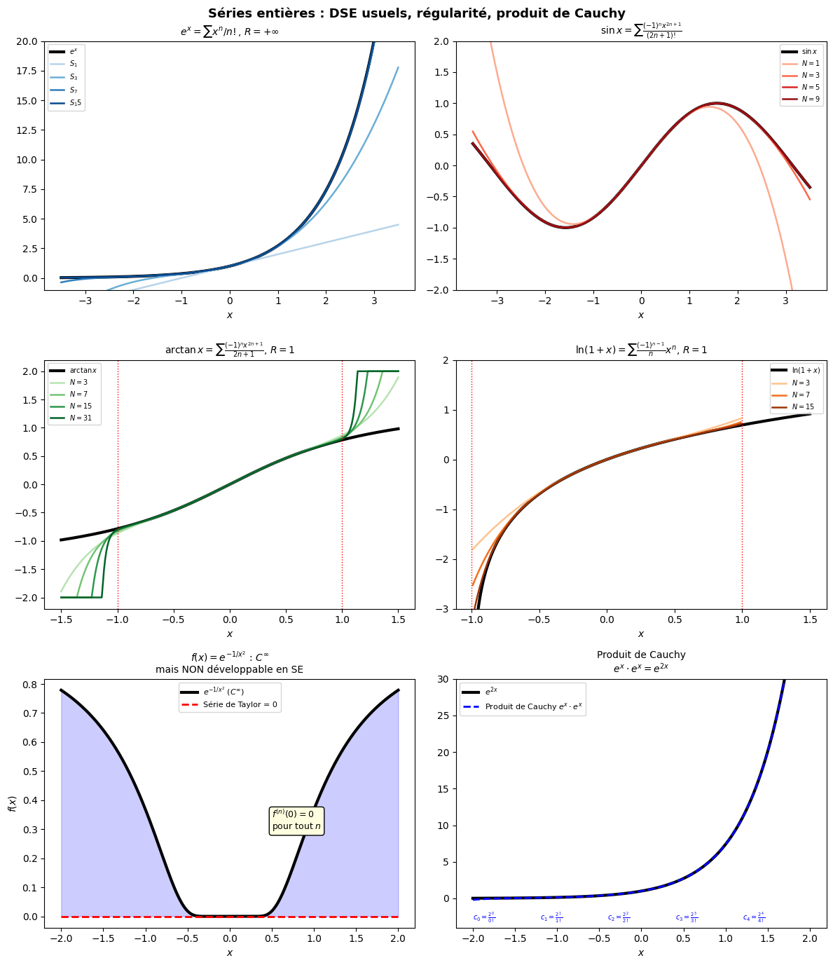
Produit de Cauchy de deux séries entières

Proposition 296

Si \(f(x) = \sum a_n x^n\) (rayon \(R_a\)) et \(g(x) = \sum b_n x^n\) (rayon \(R_b\)), alors pour \(|x| < \min(R_a, R_b)\) :

\[f(x) \cdot g(x) = \sum_{n=0}^\infty c_n x^n, \quad c_n = \sum_{k=0}^n a_k b_{n-k}\]

Proof. Pour \(|x| < \min(R_a, R_b)\) les deux séries convergent absolument. Le théorème de Mertens permet de multiplier deux séries absolument convergentes : le produit de Cauchy converge vers le produit des sommes.

Exemple 108

\(e^x \cdot e^x\) : \(c_n = \sum_{k=0}^n \frac{1}{k!(n-k)!} = \frac{1}{n!}\sum_k\binom{n}{k} = \frac{2^n}{n!}\). On retrouve \(e^{2x}\).

Exponentielle de matrice

Proposition 297 (Série exponentielle de matrice)

Pour \(A \in \mathcal{M}_n(\mathbb{C})\), la série \(e^A = \sum_{k=0}^\infty \frac{A^k}{k!}\) converge (absolument pour toute norme matricielle) et vérifie :

• \(e^0 = I_n\)

• \(AB = BA \Rightarrow e^{A+B} = e^A e^B\)

• \((e^A)^{-1} = e^{-A}\)

• \(\det(e^A) = e^{\operatorname{tr}(A)}\) (formule de Jacobi-Liouville)

Proof. Convergence : \(\|\frac{A^k}{k!}\| \leq \frac{\|A\|^k}{k!}\) et \(\sum \|A\|^k/k! = e^{\|A\|}\) converge.

\(e^{A+B} = e^A e^B\) : Par le produit de Cauchy de deux séries absolument convergentes (si \(AB = BA\), les termes commutent).

\(\det(e^A) = e^{\operatorname{tr}(A)}\) : \(A\) est triangularisable dans \(\mathbb{C}\) : si \(A = P(\lambda_i \delta_{ij} + N)P^{-1}\) (Jordan), alors \(e^A = Pe^Je^N P^{-1}\) et \(\det(e^A) = \prod_i e^{\lambda_i} = e^{\sum \lambda_i} = e^{\operatorname{tr}(A)}\).

Résumé

Concept	Formule / Propriété
Rayon de convergence	$1/R = \limsup
Lemme d’Abel	\(a_nz_0^n\) borné \(\Rightarrow\) CV absolue pour $
CV normale	Sur tout compact \(K \subset D(0,R)\)
Régularité	\(f\) est \(\mathcal{C}^\infty\) sur \(D(0,R)\)
Dérivation	Même rayon, \(f' = \sum na_nz^{n-1}\)
Intégration	Même rayon, \(\int_0^x f = \sum a_nx^{n+1}/(n+1)\)
Unicité DSE	\(a_n = f^{(n)}(0)/n!\)
\(C^\infty \not\Rightarrow\) analytique	\(e^{-1/x^2}\) : tous les \(f^{(n)}(0) = 0\)
Produit de Cauchy	\(c_n = \sum_{k=0}^n a_k b_{n-k}\)