Réduction des endomorphismes

Diagonaliser une matrice, c’est trouver le bon angle pour la regarder.

— James Joseph Sylvester

Valeurs propres et vecteurs propres

Définition 171 (Valeur propre, vecteur propre, spectre)

Soit \(f \in \mathcal{L}(E)\). Un scalaire \(\lambda \in \mathbb{K}\) est une valeur propre de \(f\) s’il existe \(v \neq 0\) tel que \(f(v) = \lambda v\).

\(v\) est un vecteur propre associé à \(\lambda\). Le sous-espace propre est \(E_\lambda = \ker(f - \lambda\,\mathrm{id})\).

Le spectre de \(f\) est \(\mathrm{Sp}(f) = \{\lambda \in \mathbb{K} \mid \lambda \text{ valeur propre}\}\).

Remarque 95

Géométriquement, les directions propres sont les directions invariantes par \(f\) : \(f\) agit comme une homothétie de rapport \(\lambda\) sur \(E_\lambda\).

Exemple 90

Endomorphisme	Valeurs propres	Vecteurs propres
\(\mathrm{id}_E\)	\(\lambda = 1\) (mult. \(n\))	Tout \(v \neq 0\)
Homothétie \(\alpha\,\mathrm{id}\)	\(\lambda = \alpha\)	Tout \(v \neq 0\)
Symétrie par rapport à \(F\)	\(1\) (sur \(F\)), \(-1\) (sur \(G\))	\(F\), \(G\)
Rotation \(\pi/2\) dans \(\mathbb{R}^2\)	Aucune sur \(\mathbb{R}\), \(\pm i\) sur \(\mathbb{C}\)	—
Dérivation sur \(\mathbb{R}[X]\)	\(0, 1, 2, \ldots\)	\(1, e^x, e^{2x}, \ldots\)

Proposition 258 (Indépendance des vecteurs propres)

Des vecteurs propres associés à des valeurs propres distinctes sont linéairement indépendants. La somme des sous-espaces propres est directe :

\[E_{\lambda_1} + \cdots + E_{\lambda_p} = E_{\lambda_1} \oplus \cdots \oplus E_{\lambda_p}.\]

Proof. Par récurrence sur \(p\). Supposons \(\sum_{i=1}^p \lambda_i v_i = 0\) (avec \(f(v_i) = \mu_i v_i\), \(\mu_i\) distincts). En appliquant \(f - \mu_p\,\mathrm{id}\) :

\[\sum_{i=1}^{p-1}(\mu_i - \mu_p)\lambda_i v_i = 0.\]

Par hypothèse de récurrence (les \(\mu_i - \mu_p \neq 0\)) : \(\lambda_i = 0\) pour \(i < p\), puis \(\lambda_p = 0\).

Polynôme caractéristique

Définition 172 (Polynôme caractéristique)

\[\chi_f(\lambda) = \det(\lambda\,\mathrm{id} - f) = \det(\lambda I_n - A).\]

C’est un polynôme de degré \(n\) en \(\lambda\) avec coefficient dominant \(1\) :

\[\chi_f(\lambda) = \lambda^n - \mathrm{tr}(A)\,\lambda^{n-1} + \cdots + (-1)^n \det(A).\]

Remarque 96

Certains auteurs définissent \(\chi_f(\lambda) = \det(A - \lambda I_n)\) (signe \((-1)^n\) modifié). Les racines sont les mêmes.

Proposition 259 (Racines et valeurs propres)

\[\lambda \in \mathrm{Sp}(f) \iff \chi_f(\lambda) = 0.\]

Les matrices semblables ont le même polynôme caractéristique.

Proof. \(\lambda\) valeur propre \(\iff\) \(\ker(f-\lambda\,\mathrm{id}) \neq \{0\}\) \(\iff\) \((f-\lambda\,\mathrm{id})\) non inversible \(\iff\) \(\det(\lambda\,\mathrm{id}-f) = 0\).

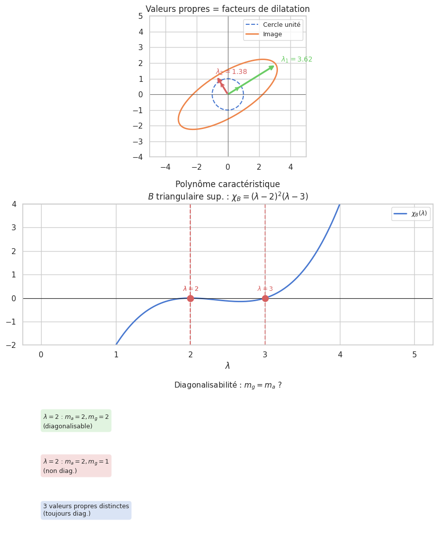
Définition 173 (Multiplicités)

Pour \(\lambda \in \mathrm{Sp}(f)\) :

• Multiplicité algébrique \(m_a(\lambda)\) : ordre de \(\lambda\) comme racine de \(\chi_f\)

• Multiplicité géométrique \(m_g(\lambda) = \dim E_\lambda\)

On a toujours \(1 \leq m_g(\lambda) \leq m_a(\lambda)\).

Show code cell source

Hide code cell source

import numpy as np
import matplotlib.pyplot as plt
import seaborn as sns
import math
from matplotlib.patches import FancyArrowPatch
from mpl_toolkits.mplot3d import proj3d

sns.set_theme(style="whitegrid", palette="muted", font_scale=1.0)

fig, axes = plt.subplots(3, 1, figsize=(9, 11))

# 1. Transformation d'une ellipse : valeurs propres = demi-axes
A = np.array([[3., 1.], [1., 2.]])
vals, vecs = np.linalg.eig(A)
theta = np.linspace(0, 2*np.pi, 200)
circle = np.vstack([np.cos(theta), np.sin(theta)])
ellipse = A @ circle

ax = axes[0]
ax.plot(circle[0], circle[1], 'C0--', lw=1.5, label='Cercle unité')
ax.plot(ellipse[0], ellipse[1], 'C1-', lw=2, label='Image')
for i, (val, vec, c) in enumerate(zip(vals, vecs.T, ['C2','C3'])):
    ax.annotate('', xy=val*vec, xytext=(0,0),
                arrowprops=dict(arrowstyle='->', color=c, lw=2.5))
    ax.annotate('', xy=vec, xytext=(0,0),
                arrowprops=dict(arrowstyle='->', color=c, lw=1.5, ls='--'))
    ax.text(val*vec[0]*1.1, val*vec[1]*1.1, f'$\\lambda_{i+1}={val:.2f}$',
            fontsize=10, color=c)
ax.set(aspect='equal', xlim=(-5,5), ylim=(-4,5),
       title='Valeurs propres = facteurs de dilatation')
ax.axhline(0, color='k', lw=0.4); ax.axvline(0, color='k', lw=0.4)
ax.legend(fontsize=9)

# 2. Polynôme caractéristique : racines
# Matrice 3x3
B = np.array([[2., 1., 0.],
              [0., 2., 1.],
              [0., 0., 3.]])
chiB = np.poly(B)  # coefficients du poly caractéristique (convention numpy)
lam = np.linspace(0, 5, 300)
chi_vals = np.polyval(chiB, lam)
roots = np.linalg.eigvals(B)

ax2 = axes[1]
ax2.plot(lam, chi_vals, 'C0-', lw=2, label='$\\chi_B(\\lambda)$')
ax2.axhline(0, color='k', lw=0.8)
for r in sorted(roots.real):
    ax2.axvline(r, color='C3', ls='--', alpha=0.7)
    ax2.scatter([r], [0], s=80, color='C3', zorder=5)
    ax2.text(r, 0.3, f'$\\lambda={r:.0f}$', ha='center', fontsize=9, color='C3')
ax2.set(xlabel='$\\lambda$', title='Polynôme caractéristique\n$B$ triangulaire sup. : $\\chi_B=(\\lambda-2)^2(\\lambda-3)$')
ax2.legend(fontsize=9)
ax2.set_ylim(-2, 4)

# 3. m_g vs m_a pour plusieurs matrices
cases = [
    ('$\\lambda=2$ : $m_a=2, m_g=2$\n(diagonalisable)', np.diag([2.,2.,3.]), 'C2'),
    ('$\\lambda=2$ : $m_a=2, m_g=1$\n(non diag.)', B, 'C3'),
    ('3 valeurs propres distinctes\n(toujours diag.)', np.array([[1.,1.,0.],[0.,2.,1.],[0.,0.,3.]]), 'C0'),
]
ax3 = axes[2]
ax3.axis('off')
ax3.set_title('Diagonalisabilité : $m_g = m_a$ ?', fontsize=11)
for i, (lbl, M, col) in enumerate(cases):
    y = 0.85 - i * 0.32
    eigs = np.linalg.eigvals(M)
    ax3.text(0.05, y, lbl, transform=ax3.transAxes, fontsize=9, va='top',
             bbox=dict(boxstyle='round,pad=0.4', facecolor=col, alpha=0.2))
    diag_str = 'Diag.' if abs(eigs[0]-eigs[1]) > 0.5 or (abs(eigs[0]-eigs[1]) < 0.1 and np.linalg.matrix_rank(M - eigs[0]*np.eye(3)) == 1) else '?'

plt.tight_layout()
plt.show()

Diagonalisation

Définition 174 (Endomorphisme diagonalisable)

\(f\) est diagonalisable s’il existe une base de \(E\) formée de vecteurs propres, i.e. sa matrice dans cette base est diagonale \(D = \mathrm{diag}(\lambda_1,\ldots,\lambda_n)\).

Proposition 260 (Caractérisations de la diagonalisabilité)

Les assertions suivantes sont équivalentes :

1. \(f\) est diagonalisable

2. \(E = \bigoplus_{\lambda \in \mathrm{Sp}(f)} E_\lambda\)

3. \(\sum_{\lambda} \dim E_\lambda = n\)

4. \(\chi_f\) est scindé sur \(\mathbb{K}\) et \(m_g(\lambda) = m_a(\lambda)\) pour tout \(\lambda\)

Proof. \((1 \Leftrightarrow 2)\) : \(f\) diagonalisable \(\Leftrightarrow\) il existe une base de vecteurs propres \(\Leftrightarrow\) \(E\) est la réunion directe des sous-espaces propres.

\((3 \Leftrightarrow 4)\) : \(\sum m_a(\lambda) = n\) (si \(\chi_f\) scindé) et \(m_g \leq m_a\) pour chaque \(\lambda\). L’égalité \(\sum m_g = n\) force \(m_g = m_a\) pour chaque \(\lambda\) et le fait que \(\chi_f\) est scindé.

Proposition 261 (Critère suffisant)

Si \(f\) a \(n = \dim E\) valeurs propres distinctes, alors \(f\) est diagonalisable.

Remarque 97

Méthode de diagonalisation :

1. Calculer \(\chi_f(\lambda) = \det(\lambda I - A)\)

2. Factoriser pour trouver les valeurs propres \(\lambda_i\) et leurs multiplicités algébriques \(m_a(\lambda_i)\)

3. Pour chaque \(\lambda_i\) : calculer \(E_{\lambda_i} = \ker(A - \lambda_i I)\) et vérifier \(\dim E_{\lambda_i} = m_a(\lambda_i)\)

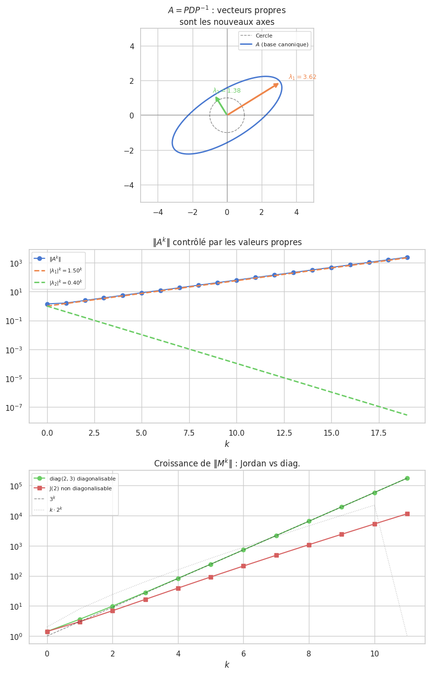
4. Former \(P\) = matrice de passage (colonnes = vecteurs propres), alors \(D = P^{-1}AP\)

Proposition 262 (Puissances d’une matrice diagonalisable)

Si \(A = PDP^{-1}\) avec \(D = \mathrm{diag}(\lambda_1,\ldots,\lambda_n)\) :

\[A^k = PD^kP^{-1} = P\,\mathrm{diag}(\lambda_1^k,\ldots,\lambda_n^k)\,P^{-1}.\]

Show code cell source

Hide code cell source

fig, axes = plt.subplots(3, 1, figsize=(9, 14))

# 1. Diagonalisation : illustration géométrique (ellipse -> axes)
A_diag = np.array([[3., 1.], [1., 2.]])
vals, P = np.linalg.eig(A_diag)
D = np.diag(vals)

theta = np.linspace(0, 2*np.pi, 200)
circle = np.vstack([np.cos(theta), np.sin(theta)])

ax = axes[0]
# Dans la base propre : A est diagonale = étirement axial
ellipse_orig = A_diag @ circle
ellipse_prop = D @ circle  # dans la base propre (cercle -> ellipse alignée)

ax.plot(circle[0], circle[1], 'k--', lw=1, alpha=0.5, label='Cercle')
ax.plot(ellipse_orig[0], ellipse_orig[1], 'C0-', lw=2, label='$A$ (base canonique)')
for i, (val, vec, c) in enumerate(zip(vals, P.T, ['C1','C2'])):
    ax.annotate('', xy=vec*val, xytext=(0,0),
                arrowprops=dict(arrowstyle='->', color=c, lw=2.5))
    ax.text(vec[0]*val*1.15, vec[1]*val*1.1,
            f'$\\lambda_{i+1}={val:.2f}$', fontsize=9, color=c)
ax.set(aspect='equal', xlim=(-5,5), ylim=(-5,5),
       title='$A = PDP^{-1}$ : vecteurs propres\nsont les nouveaux axes')
ax.axhline(0, color='k', lw=0.3); ax.axvline(0, color='k', lw=0.3)
ax.legend(fontsize=8)

# 2. Puissances de matrice par diagonalisation
A2 = np.array([[1.2, 0.8], [0.3, 0.7]])
vals2, P2 = np.linalg.eig(A2)
ks = np.arange(20)
norms = [np.linalg.norm(np.linalg.matrix_power(A2, k)) for k in ks]
norms_approx = [abs(vals2[0])**k * np.linalg.norm(P2 @ np.diag([1,0]) @ np.linalg.inv(P2))
                for k in ks]

ax2 = axes[1]
ax2.semilogy(ks, norms, 'C0o-', ms=6, label='$\\|A^k\\|$')
ax2.semilogy(ks, [abs(vals2[0])**k for k in ks], 'C1--', lw=2,
             label=f'$|\\lambda_1|^k = {abs(vals2[0]):.2f}^k$')
ax2.semilogy(ks, [abs(vals2[1])**k for k in ks], 'C2--', lw=2,
             label=f'$|\\lambda_2|^k = {abs(vals2[1]):.2f}^k$')
ax2.set(xlabel='$k$', title='$\\|A^k\\|$ contrôlé par les valeurs propres')
ax2.legend(fontsize=8)

# 3. Comparaison diagonalisable / non-diagonalisable
M_diag = np.array([[2., 0.], [0., 3.]])        # Diagonale, triviale
M_ndiag = np.array([[2., 1.], [0., 2.]])       # Jordan 2x2

ks3 = np.arange(12)
norms_d = [np.linalg.norm(np.linalg.matrix_power(M_diag, k)) for k in ks3]
norms_nd = [np.linalg.norm(np.linalg.matrix_power(M_ndiag, k)) for k in ks3]

ax3 = axes[2]
ax3.semilogy(ks3, norms_d, 'C2o-', ms=6, label='$\\mathrm{diag}(2,3)$ diagonalisable')
ax3.semilogy(ks3, norms_nd, 'C3s-', ms=6, label=r'J$(2)$ non diagonalisable')
ax3.semilogy(ks3, [3.**k for k in ks3], 'k--', lw=1, alpha=0.5, label='$3^k$')
ax3.semilogy(ks3, [2.**k * k for k in ks3 if k>0] + [1], 'gray',
             lw=1, alpha=0.5, ls=':', label='$k \\cdot 2^k$')
ax3.set(xlabel='$k$', title='Croissance de $\\|M^k\\|$ : Jordan vs diag.')
ax3.legend(fontsize=8)

plt.tight_layout()
plt.show()

Trigonalisation

Définition 175 (Matrice trigonalisable)

\(A\) est trigonalisable si \(\exists P \in GL_n(\mathbb{K}),\ T\) triangulaire sup. : \(A = PTP^{-1}\).

Proposition 263 (Critère)

\(f\) est trigonalisable \(\iff\) \(\chi_f\) est scindé sur \(\mathbb{K}\).

En particulier, toute matrice complexe est trigonalisable (d’Alembert-Gauss).

Remarque 98

Les éléments diagonaux de \(T\) sont les valeurs propres (avec multiplicités). En effet, \(\det(\lambda I - T) = \prod_i(\lambda - t_{ii})\).

Théorème de Cayley-Hamilton

Proposition 264 (Théorème de Cayley-Hamilton)

Tout endomorphisme est annulé par son propre polynôme caractéristique :

\[\chi_f(f) = 0_{\mathcal{L}(E)}.\]

Proof. (Esquisse) Sur \(\mathbb{C}\) (puis par densité), \(f\) est trigonalisable : \(A = PTP^{-1}\). \(\chi_A = \chi_T = \prod_i(\lambda - t_{ii})\). Un calcul direct montre que \(\chi_T(T) = 0\), puis \(\chi_A(A) = P\chi_T(T)P^{-1} = 0\).

Exemple 91

\(A = \begin{pmatrix}1&2\\0&3\end{pmatrix}\), \(\chi_A(\lambda) = \lambda^2 - 4\lambda + 3\).

\(A^2 - 4A + 3I = \begin{pmatrix}1&8\\0&9\end{pmatrix} - \begin{pmatrix}4&8\\0&12\end{pmatrix} + \begin{pmatrix}3&0\\0&3\end{pmatrix} = \begin{pmatrix}0&0\\0&0\end{pmatrix}\). ✓

Remarque 99

Application. Cayley-Hamilton permet de calculer \(A^{-1}\) (et plus généralement toute puissance \(A^k\)) en fonction de \(I, A, \ldots, A^{n-1}\) : \(\chi_A(A) = 0\) donne \(A^n\) en fonction des puissances inférieures.

Polynôme minimal

Définition 176 (Polynôme minimal)

Le polynôme minimal \(\mu_f\) est le polynôme annulateur unitaire de degré minimal.

Proposition 265 (Propriétés)

• \(\mu_f \mid P\) pour tout annulateur \(P\) (en particulier \(\mu_f \mid \chi_f\))

• \(\mu_f\) et \(\chi_f\) ont les mêmes racines (pas nécessairement les mêmes multiplicités)

• \(f\) diagonalisable \(\iff\) \(\mu_f\) est scindé à racines simples (lemme des noyaux)

Proof. Lemme des noyaux. Si \(\mu_f = \prod_{i=1}^p (X - \lambda_i)\) à racines distinctes, alors les \((f - \lambda_i\,\mathrm{id})\) sont premiers entre eux deux à deux, et le lemme des noyaux donne \(E = \bigoplus_i \ker(f - \lambda_i\,\mathrm{id}) = \bigoplus_i E_{\lambda_i}\).

Exemple 92

Matrice	\(\chi\)	\(\mu\)	Diag. ?
\(I_n\)	\((\lambda-1)^n\)	\(\lambda-1\)	Oui
\(\begin{pmatrix}0&1\\0&0\end{pmatrix}\)	\(\lambda^2\)	\(\lambda^2\)	Non
\(\mathrm{diag}(1,1,2)\)	\((\lambda-1)^2(\lambda-2)\)	\((\lambda-1)(\lambda-2)\)	Oui
\(\begin{pmatrix}1&1&0\\0&1&0\\0&0&2\end{pmatrix}\)	\((\lambda-1)^2(\lambda-2)\)	\((\lambda-1)^2(\lambda-2)\)	Non

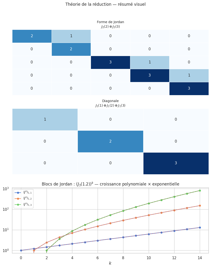
Forme de Jordan (introduction)

Définition 177 (Bloc de Jordan)

Un bloc de Jordan de taille \(k\) associé à \(\lambda\) est la matrice \(k\times k\) :

\[\begin{split}J_k(\lambda) = \begin{pmatrix} \lambda & 1 & & \\ & \lambda & \ddots & \\ & & \ddots & 1 \\ & & & \lambda \end{pmatrix}.\end{split}\]

Proposition 266 (Théorème de Jordan)

Toute matrice de \(\mathcal{M}_n(\mathbb{C})\) est semblable à une matrice de Jordan :

\[J = \mathrm{diag}(J_{k_1}(\lambda_1), J_{k_2}(\lambda_2), \ldots, J_{k_r}(\lambda_r)).\]

La décomposition est unique à permutation des blocs près.

Remarque 100

• \(f\) diagonalisable \(\iff\) tous les blocs Jordan sont de taille 1 (toutes les valeurs propres ont \(m_g = m_a\)).

• La taille du plus grand bloc de Jordan pour \(\lambda\) est l’ordre de \(\lambda\) comme racine de \(\mu_f\).

• Cayley-Hamilton : \(\chi_f = \prod_i (\lambda - \lambda_i)^{m_a(\lambda_i)}\) ; \(\mu_f = \prod_i (\lambda - \lambda_i)^{k_{\max,i}}\).

Show code cell source

Hide code cell source

fig, axes = plt.subplots(3, 1, figsize=(9, 11))

# 1. Forme de Jordan : visualisation heatmap
J_blocks = [
    (np.diag([2.,2.,3.,3.,3.]) + np.diag([1.,0.,1.,1.],1),
     'Forme de Jordan\n$J_2(2) \\oplus J_3(3)$'),
    (np.diag([1.,2.,3.]),
     'Diagonale\n$J_1(1) \\oplus J_1(2) \\oplus J_1(3)$'),
]
for ax, (J, title) in zip(axes[:2], J_blocks):
    sns.heatmap(J, ax=ax, annot=True, fmt='.0f', cmap='Blues',
                linewidths=0.5, cbar=False, annot_kws={'size': 11})
    ax.set_title(title, fontsize=10)
    ax.set_xticks([]); ax.set_yticks([])

# 2. Puissances de blocs Jordan : comportement (1+N)^k vs N^k
k_vals = np.arange(15)
lam = 1.2

# Bloc Jordan 3x3 : J = lambda*I + N
N3 = np.diag([1.,1.], k=1)
J3 = lam*np.eye(3) + N3

ax3 = axes[2]
for i in range(3):
    entries = [np.linalg.matrix_power(J3, k)[0, i] for k in k_vals]
    ax3.plot(k_vals, entries, 'o-', ms=5, label=f'$(J^k)_{{1,{i+1}}}$')

# Comportement théorique : (J^k)_{1,j} = C(k,j-1) * lambda^{k-j+1}
for j in range(1, 4):
    theo = [float(math.comb(int(k), j-1)) * lam**(k-j+1) if k >= j-1 else 0
            for k in k_vals]
    ax3.plot(k_vals, theo, '--', lw=1.5, alpha=0.6)

ax3.set(xlabel='$k$', title=f'Blocs de Jordan : $(J_3({lam}))^k$ — croissance polynomiale × exponentielle',
        yscale='log')
ax3.legend(fontsize=9)

plt.suptitle('Théorie de la réduction — résumé visuel', fontsize=12, y=1.02)
plt.tight_layout()
plt.show()

Applications importantes

Diagonalisation et systèmes récurrents

Exemple 93

Suite de Fibonacci. Posons \(X_n = \begin{pmatrix}F_{n+1}\\F_n\end{pmatrix}\). Alors \(X_n = A X_{n-1}\) avec \(A = \begin{pmatrix}1&1\\1&0\end{pmatrix}\).

\(\chi_A = \lambda^2 - \lambda - 1\), racines \(\varphi = \frac{1+\sqrt5}{2}\) et \(\hat\varphi = \frac{1-\sqrt5}{2}\).

\(P = \begin{pmatrix}\varphi&\hat\varphi\\1&1\end{pmatrix}\), \(D = \mathrm{diag}(\varphi, \hat\varphi)\), \(A^n = PD^nP^{-1}\), d’où la formule de Binet :

\[F_n = \frac{\varphi^n - \hat\varphi^n}{\sqrt{5}}.\]

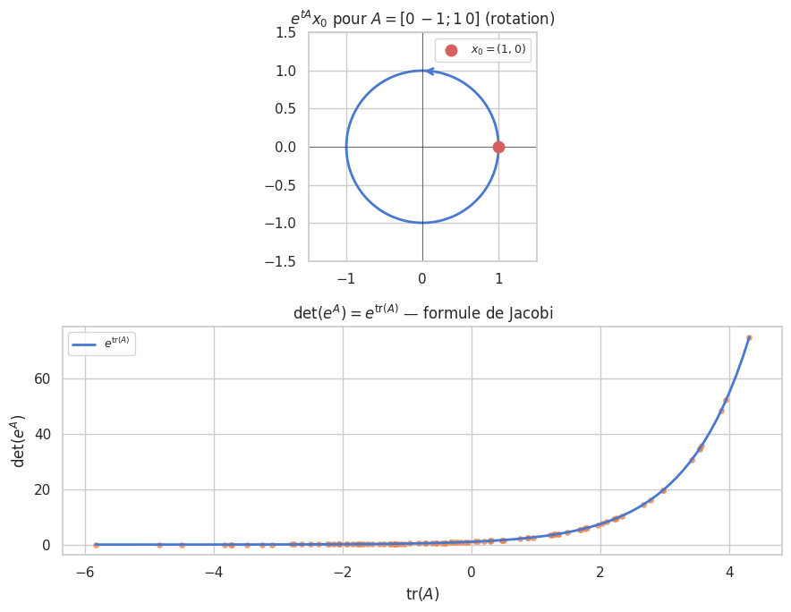
Exponentielle de matrice

Définition 178 (Exponentielle de matrice)

\[e^A = \sum_{k=0}^{+\infty} \frac{A^k}{k!} \in \mathcal{M}_n(\mathbb{K}).\]

La série converge pour toute matrice \(A\).

Proposition 267 (Propriétés)

• Si \(A = PDP^{-1}\) (diagonalisable) : \(e^A = P\,\mathrm{diag}(e^{\lambda_i})\,P^{-1}\)

• \(\det(e^A) = e^{\mathrm{tr}(A)}\) (formule de Jacobi-Liouville)

• \(e^{A+B} = e^A e^B\) si \(AB = BA\)

• \((e^{tA})' = A e^{tA}\) : solution de \(X' = AX\), \(X(0) = X_0\) est \(X(t) = e^{tA}X_0\)

Show code cell source

Hide code cell source

fig, axes = plt.subplots(2, 1, figsize=(9, 7))

# 1. Exponentielle de matrice : e^{tA} pour A diagonalisable
A_exp = np.array([[0., -1.], [1., 0.]])  # Rotation : exp(tA) = rotation d'angle t
t_vals = np.linspace(0, 2*np.pi, 200)

def mat_exp(A, t):
    """Calcule e^{tA} par diagonalisation ou série."""
    return np.array([[np.cos(t), -np.sin(t)], [np.sin(t), np.cos(t)]])

# Trajectoire d'un point sous e^{tA}
x0 = np.array([1., 0.])
trajectory = np.array([mat_exp(A_exp, t) @ x0 for t in t_vals])

ax = axes[0]
ax.plot(trajectory[:,0], trajectory[:,1], 'C0-', lw=2)
ax.scatter([x0[0]], [x0[1]], s=80, color='C3', zorder=5, label='$x_0 = (1,0)$')
ax.annotate('', xy=trajectory[50], xytext=trajectory[45],
            arrowprops=dict(arrowstyle='->', color='C0', lw=2))
ax.set(aspect='equal', xlim=(-1.5, 1.5), ylim=(-1.5, 1.5),
       title="$e^{tA}x_0$ pour $A = [0\\,-1; 1\\,0]$ (rotation)")
ax.axhline(0, color='k', lw=0.4); ax.axvline(0, color='k', lw=0.4)
ax.legend(fontsize=9)

# 2. Formule de Jacobi : det(e^A) = e^{tr(A)}
np.random.seed(3)
n_test = 100
traces = np.random.randn(n_test) * 2
det_eA = []
for tr in traces:
    A_test = np.random.randn(3,3)
    A_test = A_test + tr/3*np.eye(3) - np.trace(A_test)/3*np.eye(3)
    eA = np.zeros((3,3))
    for k in range(20):
        eA += np.linalg.matrix_power(A_test, k) / math.factorial(k)
    det_eA.append(np.linalg.det(eA))
    traces[len(det_eA)-1] = np.trace(A_test)

axes[1].scatter(traces, det_eA, s=15, alpha=0.7, color='C1')
t_line = np.linspace(min(traces), max(traces), 100)
axes[1].plot(t_line, np.exp(t_line), 'C0-', lw=2, label='$e^{\\mathrm{tr}(A)}$')
axes[1].set(xlabel='$\\mathrm{tr}(A)$', ylabel='$\\det(e^A)$',
            title='$\\det(e^A) = e^{\\mathrm{tr}(A)}$ — formule de Jacobi')
axes[1].legend(fontsize=9)

plt.tight_layout()
plt.show()