Arithmétique

Les mathématiques sont la reine des sciences, et l’arithmétique est la reine des mathématiques.

Carl Friedrich Gauss

Introduction

L’arithmétique — l’étude des propriétés des entiers — est l’un des plus anciens et des plus vivants domaines des mathématiques. Ce chapitre reprend et approfondit les notions de divisibilité, de congruences et de nombres premiers, en les inscrivant dans le cadre algébrique des anneaux. Les applications modernes — cryptographie RSA, codes correcteurs d’erreurs — reposent directement sur ces résultats.

Show code cell source

Hide code cell source

import numpy as np
import matplotlib.pyplot as plt
import seaborn as sns
from math import gcd

sns.set_theme(style="whitegrid", palette="muted", font_scale=1.1)

fig, axes = plt.subplots(3, 1, figsize=(9, 14))

# 1. Crible d'Eratosthène visualisé
ax = axes[0]
N = 100
sieve = np.ones(N+1, dtype=bool)
sieve[0] = sieve[1] = False
for i in range(2, int(N**0.5)+1):
    if sieve[i]:
        sieve[i*i::i] = False
grid = sieve[1:N+1].reshape(10, 10)
im = ax.imshow(grid, cmap='RdYlGn', aspect='auto')
for i in range(10):
    for j in range(10):
        n = i*10 + j + 1
        color = 'white' if grid[i,j] else 'gray'
        ax.text(j, i, str(n), ha='center', va='center', fontsize=8,
                color=color, fontweight='bold' if grid[i,j] else 'normal')
ax.set_xticks([]); ax.set_yticks([])
ax.set_title('Crible d\'Ératosthène (1–100)\nVert = premier')

# 2. Algorithme d'Euclide : spirale de rectangles
ax = axes[1]
a, b = 144, 89  # Fibonacci, gcd=1
colors_e = plt.cm.viridis(np.linspace(0.2, 0.9, 10))
x0, y0 = 0, 0
steps_e = []
aa, bb = a, b
while bb:
    q, r = aa // bb, aa % bb
    steps_e.append((aa, bb, q, r))
    aa, bb = bb, r

# Dessiner les rectangles de l'algorithme d'Euclide géométrique
x, y, w, h = 0, 0, a, b
horizontal = True
for k, (aa, bb, q, r) in enumerate(steps_e):
    c = colors_e[k % len(colors_e)]
    for qi in range(q):
        if horizontal:
            rect = plt.Rectangle((x + qi*bb, y), bb, bb, fc=c, ec='white', alpha=0.7)
        else:
            rect = plt.Rectangle((x, y + qi*aa), aa, aa, fc=c, ec='white', alpha=0.7)
        ax.add_patch(rect)
    if horizontal:
        x += q * bb
        w = bb; h = aa - q*bb
    else:
        y += q * aa
        h = aa; w = bb - q*aa
    horizontal = not horizontal
ax.set_xlim(0, a); ax.set_ylim(0, b)
ax.set_aspect('equal')
ax.set_title(f'Euclide géométrique : $\\mathrm{{pgcd}}({a}, {b}) = {gcd(a,b)}$\n(Nombres de Fibonacci)')
ax.set_xlabel('x'); ax.set_ylabel('y')

# 3. Théorème des nombres premiers : pi(x) vs x/ln(x)
ax = axes[2]
xs = np.arange(2, 500)
pi_x = np.array([np.sum(sieve[:x]) for x in xs])
approx = xs / np.log(xs)
li_x = np.array([np.sum(1/np.log(np.arange(2, x+1))) for x in xs])  # Li(x)
ax.plot(xs, pi_x, 'steelblue', lw=2, label='$\\pi(x)$')
ax.plot(xs, approx, 'tomato', lw=1.5, linestyle='--', label='$x/\\ln x$')
ax.plot(xs, li_x, 'gold', lw=1.5, linestyle=':', label='$\\mathrm{Li}(x)$')
ax.set_xlabel('$x$'); ax.set_ylabel('Nombre de premiers')
ax.set_title('Th. des nombres premiers\n$\\pi(x) \\sim x/\\ln x \\sim \\mathrm{Li}(x)$')
ax.legend()

plt.tight_layout()
plt.show()

Divisibilité dans \(\mathbb{Z}\)

Définition 261 (Divisibilité)

Soit \(a, b \in \mathbb{Z}\). On dit que \(a\) divise \(b\), noté \(a \mid b\), s’il existe \(k \in \mathbb{Z}\) tel que \(b = ka\).

Théorème 59 (Division euclidienne)

Pour tout \(a \in \mathbb{Z}\) et \(b \in \mathbb{Z}^*\), il existe un unique couple \((q, r) \in \mathbb{Z} \times \mathbb{N}\) tel que

\[a = bq + r \quad \text{et} \quad 0 \leq r < |b|\]

Proof. Existence : L’ensemble \(E = \{a - bk : k \in \mathbb{Z}\} \cap \mathbb{N}\) est non vide (prendre \(k\) assez négatif). Soit \(r = \min E\), obtenu pour un certain \(q\). Par construction \(r \geq 0\). Si \(r \geq |b|\), alors \(r - |b| \geq 0\) serait dans \(E\) et serait \(< r\), contradiction. Donc \(r < |b|\).

Unicité : Si \(bq_1 + r_1 = bq_2 + r_2\) avec \(0 \leq r_1, r_2 < |b|\), alors \(b(q_1 - q_2) = r_2 - r_1\). Comme \(|r_2 - r_1| < |b|\), on a \(q_1 = q_2\) puis \(r_1 = r_2\).

PGCD et algorithme d’Euclide

Définition 262 (PGCD)

Le plus grand commun diviseur de \(a, b \in \mathbb{Z}\) (non tous deux nuls) est le plus grand entier positif divisant \(a\) et \(b\). On le note \(\pgcd(a, b)\).

Théorème 60 (PGCD et idéaux)

\(\pgcd(a, b)\) est l’unique générateur positif de l’idéal \(a\mathbb{Z} + b\mathbb{Z}\). Autrement dit, \(\pgcd(a, b)\mathbb{Z} = a\mathbb{Z} + b\mathbb{Z}\).

Proof. L’idéal \(I = a\mathbb{Z} + b\mathbb{Z} = \{au + bv : u, v \in \mathbb{Z}\}\) est principal (\(\mathbb{Z}\) est principal) : \(I = d\mathbb{Z}\) pour un \(d \geq 0\). Comme \(a, b \in I\), \(d \mid a\) et \(d \mid b\). Si \(c \mid a\) et \(c \mid b\), alors \(c \mid (au + bv)\) pour tous \(u, v\), donc \(c \mid d\). Ainsi \(d = \pgcd(a, b)\).

Corollaire 3 (Identité de Bézout)

Il existe \(u, v \in \mathbb{Z}\) tels que \(au + bv = \pgcd(a, b)\).

En particulier, \(\pgcd(a, b) = 1\) (premiers entre eux) si et seulement si \(\exists u, v \in \mathbb{Z}, \; au + bv = 1\).

Théorème 61 (Algorithme d’Euclide)

\(\pgcd(a, b)\) se calcule par divisions euclidiennes successives :

\[a = bq_0 + r_0, \quad b = r_0 q_1 + r_1, \quad r_0 = r_1 q_2 + r_2, \quad \ldots\]

La suite des restes est strictement décroissante dans \(\mathbb{N}\). Le dernier reste non nul est \(\pgcd(a, b)\).

Proof. \(\pgcd(a, b) = \pgcd(b, r_0)\) car \(a = bq_0 + r_0 \implies\) (diviseurs communs de \(a, b\)) = (diviseurs communs de \(b, r_0\)). Par récurrence : \(\pgcd(a, b) = \pgcd(r_{k-1}, r_k)\). Quand \(r_{k+1} = 0\) : \(\pgcd(r_{k-1}, r_k) = r_k\).

Exemple 144

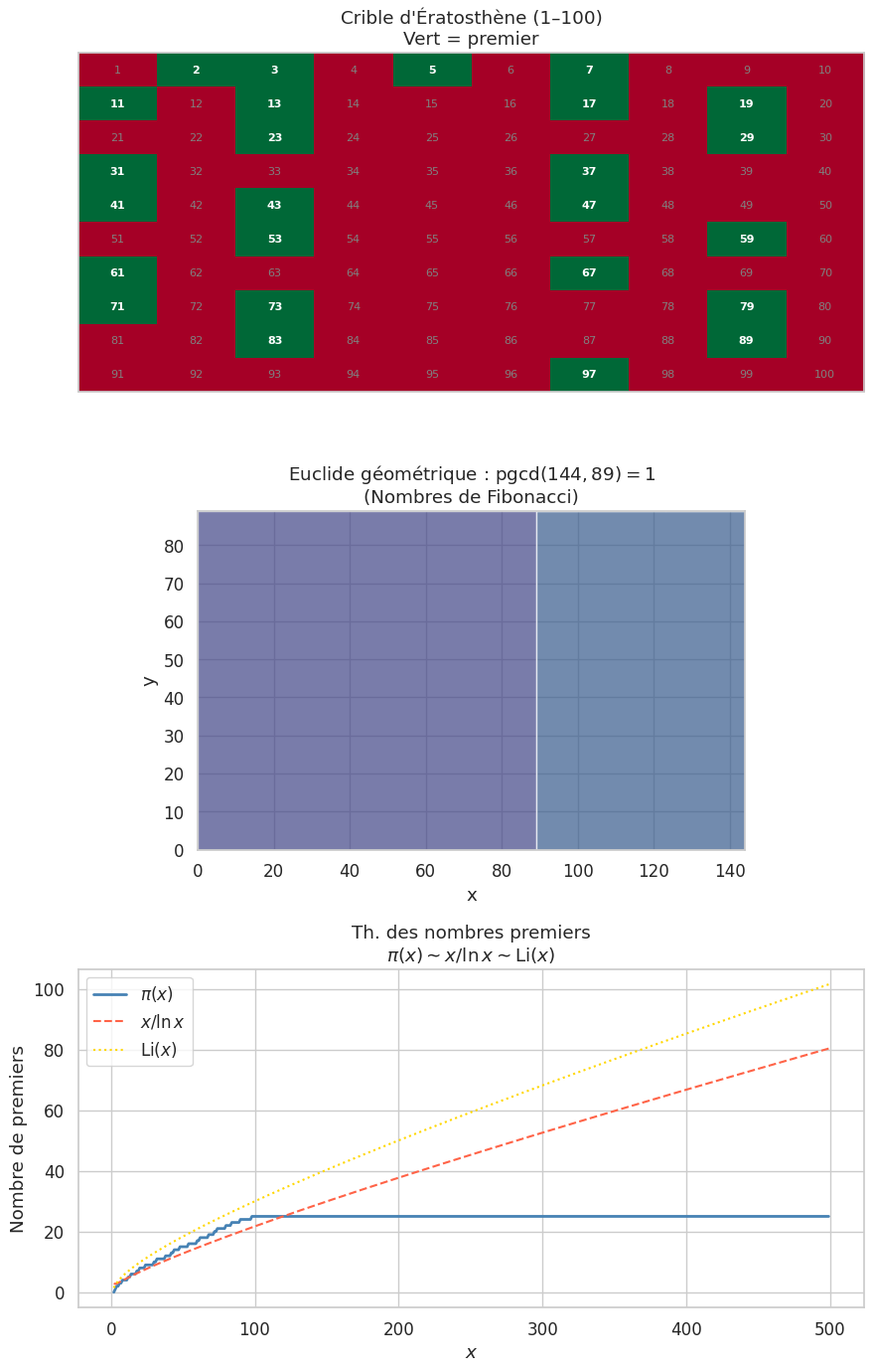
\(\pgcd(252, 198)\) : \(252 = 1 \times 198 + 54\), \(198 = 3 \times 54 + 36\), \(54 = 1 \times 36 + 18\), \(36 = 2 \times 18\). Donc \(\pgcd(252, 198) = 18\).

Bézout (remontée) : \(18 = 54 - 36 = 54 - (198 - 3\times 54) = 4\times 54 - 198 = 4(252 - 198) - 198 = 4\times 252 - 5\times 198\).

Théorème 62 (Lemme de Gauss)

Si \(a \mid bc\) et \(\pgcd(a, b) = 1\), alors \(a \mid c\).

Proof. Par Bézout, \(au + bv = 1\). En multipliant par \(c\) : \(acu + bcv = c\). Or \(a \mid acu\) et \(a \mid bcv\) (car \(a \mid bc\)), donc \(a \mid c\).

Proposition 315 (PPCM)

Le plus petit commun multiple \(\mathrm{ppcm}(a, b)\) vérifie \(\mathrm{ppcm}(a, b) \cdot \pgcd(a, b) = |ab|\).

Nombres premiers

Définition 263 (Nombre premier)

Un entier \(p \geq 2\) est premier s’il n’a pour diviseurs positifs que \(1\) et \(p\).

Théorème 63 (Théorème fondamental de l’arithmétique)

Tout entier \(n \geq 2\) se décompose de manière unique en produit de nombres premiers :

\[n = p_1^{\alpha_1} p_2^{\alpha_2} \cdots p_k^{\alpha_k}\]

avec \(p_1 < p_2 < \cdots < p_k\) premiers et \(\alpha_i \geq 1\).

Proof. Existence : Par récurrence forte. Si \(n\) est premier, fini. Sinon \(n = ab\) avec \(1 < a, b < n\), et par hypothèse \(a, b\) sont produits de premiers.

Unicité : Supposons deux décompositions. Si \(p\) premier divise \(q_1^{\beta_1} \cdots q_l^{\beta_l}\), par le lemme d’Euclide (si \(p \mid ab\), alors \(p \mid a\) ou \(p \mid b\) — car \((p)\) est un idéal premier dans \(\mathbb{Z}\)), \(p\) divise un \(q_j\), et comme \(q_j\) est premier, \(p = q_j\). On simplifie et on itère.

Théorème 64 (Infinité des nombres premiers (Euclide))

Il existe une infinité de nombres premiers.

Proof. Supposons qu’il n’y ait qu’un nombre fini de premiers \(p_1, \ldots, p_k\). Posons \(N = p_1 p_2 \cdots p_k + 1\). Aucun \(p_i\) ne divise \(N\) (car \(N \equiv 1 [p_i]\)). Mais \(N \geq 2\) a un diviseur premier, qui n’est pas dans la liste. Contradiction.

Théorème 65 (Théorème des nombres premiers)

\[\pi(x) = |\{p \leq x : p \text{ premier}\}| \sim \frac{x}{\ln x} \sim \mathrm{Li}(x) = \int_2^x \frac{dt}{\ln t}\]

L’approximation \(\mathrm{Li}(x)\) est plus précise. Ce théorème a été démontré indépendamment par Hadamard et de la Vallée Poussin en 1896.

Congruences

Définition 264 (Congruence)

Soit \(n \geq 1\). On dit que \(a \equiv b [n]\) si \(n \mid (a - b)\).

Proposition 316

La congruence modulo \(n\) est une relation d’équivalence compatible avec \(+\) et \(\times\). Les classes d’équivalence forment l’anneau \(\mathbb{Z}/n\mathbb{Z}\).

Théorème 66 (Petit théorème de Fermat)

Si \(p\) est premier et \(p \nmid a\), alors

\[a^{p-1} \equiv 1 [p]\]

Proof. Les éléments \(a, 2a, \ldots, (p-1)a\) sont tous distincts modulo \(p\) (si \(ia \equiv ja\), alors \(p \mid (i-j)a\), et \(p \nmid a\) donc \(p \mid (i-j)\), impossible pour \(0 < |i-j| < p\)). Ils forment une permutation de \(\{1, 2, \ldots, p-1\}\) modulo \(p\).

En prenant le produit : \(a^{p-1}(p-1)! \equiv (p-1)! [p]\). Comme \(p \nmid (p-1)!\), on peut simplifier : \(a^{p-1} \equiv 1 [p]\).

Théorème 67 (Théorème d’Euler)

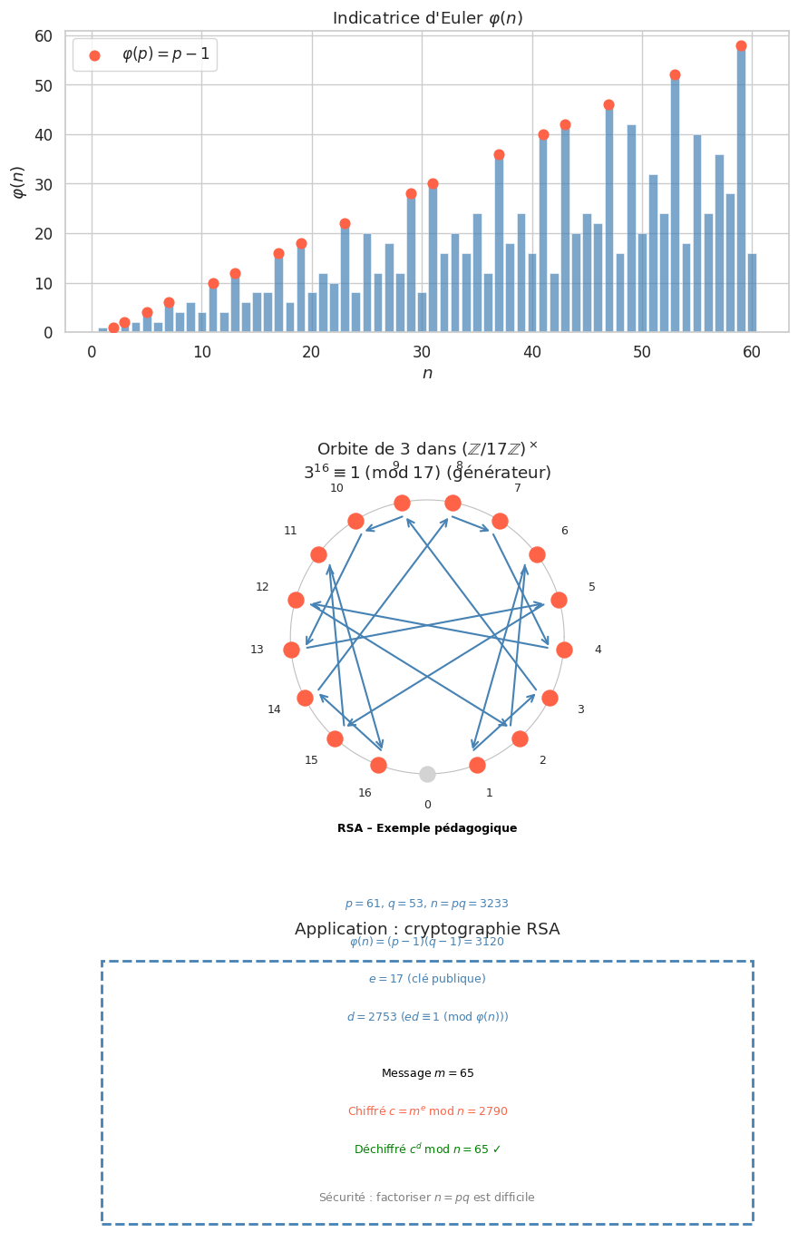
Si \(\pgcd(a, n) = 1\), alors \(a^{\varphi(n)} \equiv 1 [n]\), où \(\varphi(n) = |(\mathbb{Z}/n\mathbb{Z})^\times|\) est l”indicatrice d’Euler.

Proof. \((\mathbb{Z}/n\mathbb{Z})^\times\) est un groupe de cardinal \(\varphi(n)\). L’ordre de \(\bar{a}\) divise \(\varphi(n)\) (théorème de Lagrange), donc \(a^{\varphi(n)} \equiv 1\).

Proposition 317 (Calcul de \(\varphi(n)\))

• \(\varphi(p) = p - 1\) pour \(p\) premier

• \(\varphi(p^k) = p^{k-1}(p - 1)\)

• Multiplicativité : \(\pgcd(m, n) = 1 \implies \varphi(mn) = \varphi(m)\varphi(n)\)

• Formule générale : \(\varphi(n) = n \prod_{p \mid n} \left(1 - \frac{1}{p}\right)\)

Proof. \(\varphi(p^k) = p^{k-1}(p-1)\) : Les entiers de \(\{1, \ldots, p^k\}\) non premiers avec \(p^k\) sont exactement les multiples de \(p\) : il y en a \(p^{k-1}\). Donc \(\varphi(p^k) = p^k - p^{k-1}\).

Multiplicativité : Découle du théorème chinois des restes : \((\mathbb{Z}/mn\mathbb{Z})^\times \cong (\mathbb{Z}/m\mathbb{Z})^\times \times (\mathbb{Z}/n\mathbb{Z})^\times\).

Show code cell source

Hide code cell source

fig, axes = plt.subplots(3, 1, figsize=(9, 14))

# 1. Visualisation de phi(n) et ses propriétés
ax = axes[0]
ns = np.arange(1, 61)
from sympy import totient
phi_vals = np.array([int(totient(int(n))) for n in ns])
ax.bar(ns, phi_vals, color='steelblue', alpha=0.7, edgecolor='white', linewidth=0.5)
# Mettre en evidence les premiers p : phi(p) = p-1
primes_60 = [n for n in ns if all(n % d != 0 for d in range(2, int(n**0.5)+1)) and n > 1]
phi_primes = [int(totient(int(p))) for p in primes_60]
ax.scatter(primes_60, phi_primes, color='tomato', s=60, zorder=5, label='$\\varphi(p)=p-1$')
ax.set_xlabel('$n$'); ax.set_ylabel('$\\varphi(n)$')
ax.set_title('Indicatrice d\'Euler $\\varphi(n)$')
ax.legend()

# 2. Congruences et orbites : a^k mod n
ax = axes[1]
a_orb, n_orb = 3, 17
orbit = [(a_orb**k) % n_orb for k in range(n_orb)]
# Trouver la periode
period = next(k for k in range(1, n_orb) if (a_orb**k) % n_orb == 1)
theta_orb = [x * 2*np.pi/n_orb - np.pi/2 for x in range(n_orb)]
xs_orb = [np.cos(t) for t in theta_orb]
ys_orb = [np.sin(t) for t in theta_orb]
ax.plot(np.cos(np.linspace(0,2*np.pi,300)), np.sin(np.linspace(0,2*np.pi,300)), 'gray', lw=0.8, alpha=0.5)
# Marquer les elements de l'orbite
orbit_set = set(orbit[:period])
for x in range(n_orb):
    xk, yk = xs_orb[x], ys_orb[x]
    color = 'tomato' if x in orbit_set else 'lightgray'
    ax.scatter([xk], [yk], s=150, color=color, zorder=5)
    ax.text(xk*1.25, yk*1.25, str(x), ha='center', fontsize=9)
# Tracer les fleches
for k in range(period):
    src = orbit[k]; dst = orbit[k+1] if k+1 < period else orbit[0]
    ax.annotate('', xy=(xs_orb[dst]*0.9, ys_orb[dst]*0.9),
                xytext=(xs_orb[src]*0.9, ys_orb[src]*0.9),
                arrowprops=dict(arrowstyle='->', color='steelblue', lw=1.5))
ax.set_aspect('equal'); ax.axis('off')
ax.set_title(f'Orbite de $3$ dans $(\\mathbb{{Z}}/17\\mathbb{{Z}})^\\times$\n$3^{{{period}}} \\equiv 1 \\;(\\mathrm{{mod}}\\;17)$ (générateur)')

# 3. RSA : visualisation du chiffrement
ax = axes[2]
ax.set_xlim(0, 10); ax.set_ylim(0, 8); ax.axis('off')

# Parametres RSA pedagogiques
p_rsa, q_rsa = 61, 53
n_rsa = p_rsa * q_rsa
phi_n = (p_rsa-1)*(q_rsa-1)
e_rsa = 17
d_rsa = pow(e_rsa, -1, phi_n)  # inverse modulaire

m_rsa = 65
c_rsa = pow(m_rsa, e_rsa, n_rsa)
m_dec = pow(c_rsa, d_rsa, n_rsa)

lines = [
    ('RSA – Exemple pédagogique', 11, 'black', True),
    ('', 9.5, 'gray', False),
    (f'$p={p_rsa}$, $q={q_rsa}$, $n=pq={n_rsa}$', 9, 'steelblue', False),
    (f'$\\varphi(n)=(p-1)(q-1)={phi_n}$', 8, 'steelblue', False),
    (f'$e={e_rsa}$ (clé publique)', 7, 'steelblue', False),
    (f'$d={d_rsa}$ ($ed\\equiv 1 \\;(\\mathrm{{mod}}\\;\\varphi(n))$)', 6, 'steelblue', False),
    ('', 5, 'gray', False),
    (f'Message $m={m_rsa}$', 4.5, 'black', False),
    (f'Chiffré $c = m^e \\;\\mathrm{{mod}}\\; n = {c_rsa}$', 3.5, 'tomato', False),
    (f'Déchiffré $c^d \\;\\mathrm{{mod}}\\; n = {m_dec}$ \u2713', 2.5, 'green', False),
    ('Sécurité : factoriser $n=pq$ est difficile', 1.2, 'gray', False),
]
for (text, y, color, bold) in lines:
    ax.text(5, y, text, ha='center', va='center', fontsize=9,
            color=color, fontweight='bold' if bold else 'normal')
rect = plt.Rectangle((0.5, 0.5), 9, 7, fill=False, edgecolor='steelblue', lw=2, linestyle='--')
ax.add_patch(rect)
ax.set_title('Application : cryptographie RSA')

plt.tight_layout()
plt.show()

Théorème chinois des restes

Théorème 68 (Théorème chinois des restes)

Soit \(n_1, \ldots, n_k\) des entiers deux à deux premiers entre eux. Alors

\[\mathbb{Z}/(n_1 \cdots n_k)\mathbb{Z} \cong \mathbb{Z}/n_1\mathbb{Z} \times \cdots \times \mathbb{Z}/n_k\mathbb{Z}\]

Pour tous \(a_1, \ldots, a_k\), le système \(x \equiv a_i [n_i]\) admet une unique solution modulo \(n_1 \cdots n_k\).

Proof. Le morphisme \(\varphi : \mathbb{Z} \to \prod \mathbb{Z}/n_i\mathbb{Z}\), \(x \mapsto (x \bmod n_1, \ldots, x \bmod n_k)\) a pour noyau \(n_1 \cdots n_k \mathbb{Z}\) (car les \(n_i\) sont premiers entre eux deux à deux). Les deux anneaux ont même cardinal \(n_1 \cdots n_k\), donc \(\varphi\) est surjectif.

Construction explicite : Posons \(N = n_1 \cdots n_k\) et \(N_i = N/n_i\). Comme \(\pgcd(N_i, n_i) = 1\), par Bézout il existe \(M_i\) tel que \(N_i M_i \equiv 1 [n_i]\). Alors \(x = \sum_{i=1}^k a_i N_i M_i [N]\) est la solution.

Exemple 145

Résoudre \(x \equiv 2 [3]\) et \(x \equiv 3 [5]\). \(N = 15\), \(N_1 = 5\), \(N_2 = 3\). \(5^{-1} \equiv 2 [3]\) (car \(5 \times 2 = 10 \equiv 1\)). \(3^{-1} \equiv 2 [5]\) (car \(3 \times 2 = 6 \equiv 1\)). \(x \equiv 2 \times 5 \times 2 + 3 \times 3 \times 2 = 20 + 18 = 38 \equiv 8 [15]\). Vérification : \(8 = 2 \times 3 + 2\) ✓, \(8 = 1 \times 5 + 3\) ✓.

Application : cryptographie RSA

Remarque 132

Le système RSA (Rivest-Shamir-Adleman, 1977) est la première démonstration pratique de la cryptographie à clé publique. Son fondement mathématique repose entièrement sur l’arithmétique modulaire.

Génération des clés :

1. Choisir deux grands premiers \(p, q\) et poser \(n = pq\)

2. Calculer \(\varphi(n) = (p-1)(q-1)\)

3. Choisir \(e\) avec \(\pgcd(e, \varphi(n)) = 1\)

4. Calculer \(d \equiv e^{-1} [\varphi(n)]\) par l’algorithme d’Euclide étendu

Clé publique : \((n, e)\). Clé privée : \(d\).

Chiffrement : \(c \equiv m^e [n]\) (rapide par exponentiation rapide). Déchiffrement : \(m \equiv c^d [n]\).

Correction : Si \(\pgcd(m, n) = 1\), par Euler : \(m^{ed} = m^{1 + k\varphi(n)} = m \cdot (m^{\varphi(n)})^k \equiv m \cdot 1^k = m [n]\).

Sécurité : repose sur la difficulté de factoriser \(n = pq\) (aucun algorithme polynomial connu).

Résumé

Concept	Propriété clé
Division euclidienne	\(a = bq + r\), $0 \leq r <
PGCD	\(\pgcd(a,b)\mathbb{Z} = a\mathbb{Z} + b\mathbb{Z}\) (idéal)
Bézout	\(\pgcd(a,b) = 1 \iff \exists u,v, \; au + bv = 1\)
Gauss	\(a \mid bc\) et \(\pgcd(a,b) = 1 \implies a \mid c\)
Fondamental	Décomposition unique en premiers
Fermat	\(a^{p-1} \equiv 1 [p]\) (preuve par produit)
Euler	\(a^{\varphi(n)} \equiv 1 [n]\) si \(\pgcd(a,n) = 1\)
\(\varphi(n)\)	\(n \prod_{p \mid n}(1 - 1/p)\), multiplicative
Chinois	\(\pgcd(m,n)=1 \implies \mathbb{Z}/mn\mathbb{Z} \cong \mathbb{Z}/m\mathbb{Z} \times \mathbb{Z}/n\mathbb{Z}\)
RSA	\(c = m^e \bmod n\), \(m = c^d \bmod n\), sécurité = factorisation