Statistiques

Tous les modèles sont faux, mais certains sont utiles.

George E. P. Box

Introduction

La théorie des probabilités étudie les propriétés de phénomènes aléatoires dont le modèle est connu. La statistique résout le problème inverse : à partir de données observées, inférer les caractéristiques du modèle sous-jacent. Ce chapitre introduit les outils fondamentaux : estimation ponctuelle, borne de Cramér-Rao, intervalles de confiance et tests d’hypothèses.

Show code cell source

Hide code cell source

import numpy as np
import matplotlib.pyplot as plt
import seaborn as sns
from scipy import stats

sns.set_theme(style="whitegrid", palette="muted", font_scale=1.1)

fig, axes = plt.subplots(3, 1, figsize=(9, 14))

# 1. Biais vs variance : compromis estimateur
ax = axes[0]
ax.set_xlim(-0.5, 10.5); ax.set_ylim(-0.5, 10.5); ax.set_aspect('equal')
ax.axvline(5, color='tomato', lw=1.5, linestyle='--', alpha=0.7, label='Vraie valeur $\\theta=5$')
ax.axhline(5, color='tomato', lw=1.5, linestyle='--', alpha=0.7)

np.random.seed(42)
# Sans biais, grande variance
pts_A = np.random.normal(5, 1.5, 50)
pts_B_x = np.random.normal(5, 1.5, 50)
pts_A_y = np.random.normal(5, 1.5, 50)
ax.scatter(pts_B_x, pts_A_y, alpha=0.5, color='steelblue', s=30, label='Sans biais, grande var.')
# Biaisé, petite variance
pts_C = np.random.normal(7, 0.5, 50)
pts_D = np.random.normal(7, 0.5, 50)
ax.scatter(pts_C, pts_D, alpha=0.5, color='gold', s=30, label='Biaisé, petite var.')
ax.scatter([5], [5], color='tomato', s=200, marker='*', zorder=10)
ax.set_xlabel('Réalisation 1'); ax.set_ylabel('Réalisation 2')
ax.set_title('Compromis biais-variance\n★ = vraie valeur')
ax.legend(fontsize=8)

# 2. Vraisemblance pour N(mu, sigma^2=1)
ax = axes[1]
np.random.seed(7)
data = np.random.normal(2.5, 1, 20)
mu_grid = np.linspace(-1, 6, 300)
log_lik = np.array([-0.5*np.sum((data - mu)**2) for mu in mu_grid])
log_lik -= log_lik.max()
ax.plot(mu_grid, np.exp(log_lik), 'steelblue', lw=2.5, label='Vraisemblance $L(\\mu)$')
ax.axvline(data.mean(), color='tomato', lw=2, linestyle='--',
           label=f'EMV $\\hat{{\\mu}}=\\bar{{x}}={data.mean():.2f}$')
ax.axvline(2.5, color='gold', lw=2, linestyle=':', label='Vraie valeur $\\mu=2.5$')
ax.fill_between(mu_grid, 0, np.exp(log_lik), alpha=0.15, color='steelblue')
ax.set_xlabel('$\\mu$'); ax.set_ylabel('$L(\\mu)$ (normalisée)')
ax.set_title('Vraisemblance $\\mathcal{N}(\\mu, 1)$\n$n=20$ observations')
ax.legend(fontsize=9)

# 3. Intervalles de confiance : simulation
ax = axes[2]
np.random.seed(0)
true_mu = 3; true_sigma = 1; n_ic = 30; n_sim_ic = 40
z95 = 1.96
n_cover = 0
for i in range(n_sim_ic):
    sample = np.random.normal(true_mu, true_sigma, n_ic)
    xbar = sample.mean()
    se = true_sigma / np.sqrt(n_ic)
    lo, hi = xbar - z95*se, xbar + z95*se
    contains = lo <= true_mu <= hi
    n_cover += int(contains)
    color = 'steelblue' if contains else 'tomato'
    ax.plot([lo, hi], [i, i], color=color, lw=1.5, alpha=0.8)
    ax.scatter([xbar], [i], color=color, s=20, zorder=5)
ax.axvline(true_mu, color='black', lw=1.5, linestyle='--', label=f'$\\mu={true_mu}$')
ax.set_xlabel('$\\mu$'); ax.set_ylabel('Simulation')
ax.set_title(f'Intervalles de confiance 95%\n{n_cover}/{n_sim_ic} contiennent $\\mu$'
             f' (attendu: {int(0.95*n_sim_ic)})')
ax.legend(fontsize=9)

plt.tight_layout()
plt.show()

Cadre statistique

Définition 296 (Modèle statistique)

Un modèle statistique est un triplet \((\mathcal{X}, \mathcal{A}, (P_\theta)_{\theta \in \Theta})\) où :

• \(\mathcal{X}\) est l”espace des observations

• \((P_\theta)_{\theta \in \Theta}\) est une famille de probabilités paramétrisée par \(\theta \in \Theta\)

Le modèle est paramétrique si \(\Theta \subset \mathbb{R}^d\).

Définition 297 (Échantillon et statistique)

Un échantillon de taille \(n\) est \((X_1, \ldots, X_n)\) i.i.d. de loi \(P_\theta\).

Une statistique est une fonction mesurable \(T = T(X_1, \ldots, X_n)\) ne dépendant pas de \(\theta\).

Exemple 159

• Moyenne empirique \(\bar{X}_n = \frac{1}{n}\sum X_i\)

• Variance empirique \(S_n^2 = \frac{1}{n}\sum(X_i - \bar{X}_n)^2\) (biaisée)

• Variance corrigée \(S_n'^2 = \frac{1}{n-1}\sum(X_i - \bar{X}_n)^2\) (sans biais)

• Maximum \(X_{(n)} = \max(X_1, \ldots, X_n)\), minimum \(X_{(1)}\)

Estimation ponctuelle

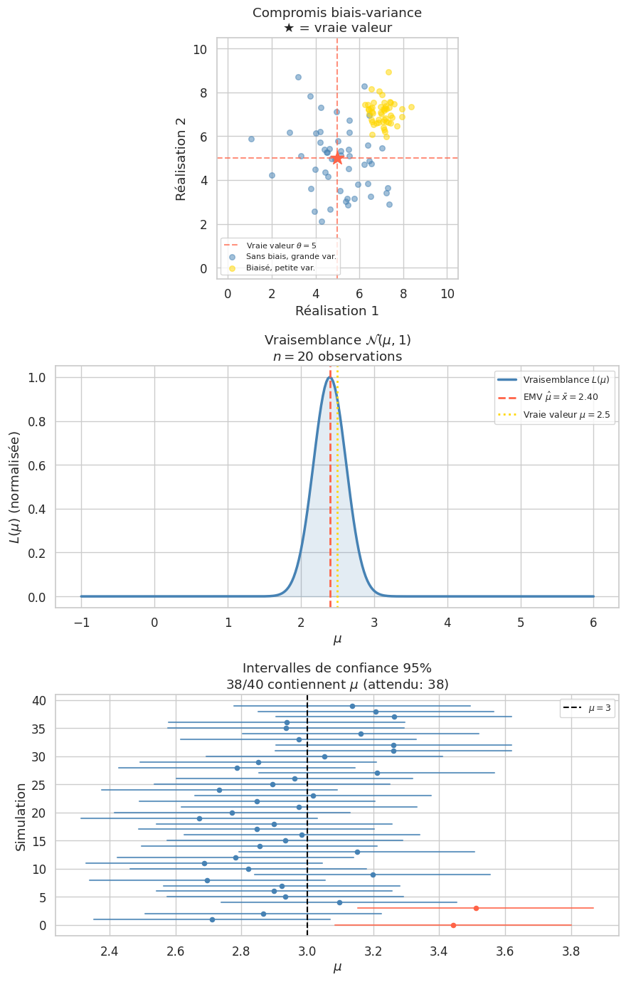
Définition 298 (Estimateur : biais et qualité)

Un estimateur de \(\theta\) est une statistique \(\hat{\theta}_n = T(X_1, \ldots, X_n)\) destinée à approcher \(\theta\).

• Sans biais : \(\mathbb{E}_\theta[\hat{\theta}_n] = \theta\) pour tout \(\theta\)

• Biais : \(b(\hat{\theta}_n) = \mathbb{E}_\theta[\hat{\theta}_n] - \theta\)

• Convergent (consistent) : \(\hat{\theta}_n \xrightarrow{\mathbb{P}} \theta\)

• EQM : \(\text{EQM}(\hat{\theta}_n) = \mathbb{E}[(\hat{\theta}_n - \theta)^2] = \text{Var}(\hat{\theta}_n) + b(\hat{\theta}_n)^2\)

Exemple 160

Variance empirique biaisée : \(\mathbb{E}[S_n^2] = \frac{n-1}{n}\sigma^2 \neq \sigma^2\).

Variance corrigée : \(\mathbb{E}[S_n'^2] = \sigma^2\) ✓.

Proof. \(\sum(X_i - \bar{X})^2 = \sum X_i^2 - n\bar{X}^2\). \(\mathbb{E}[\sum X_i^2] = n(\sigma^2 + \mu^2)\). \(\mathbb{E}[n\bar{X}^2] = n(\sigma^2/n + \mu^2) = \sigma^2 + n\mu^2\). \(\mathbb{E}[\sum(X_i - \bar{X})^2] = (n-1)\sigma^2\). Donc \(\mathbb{E}[S_n^2] = (n-1)\sigma^2/n\).

Borne de Cramér-Rao

Définition 299 (Information de Fisher)

Pour un modèle régulier à densité \(f_\theta\), l”information de Fisher est

\[I(\theta) = \mathbb{E}_\theta\!\left[\left(\frac{\partial}{\partial\theta}\ln f_\theta(X)\right)^2\right] = -\mathbb{E}_\theta\!\left[\frac{\partial^2}{\partial\theta^2}\ln f_\theta(X)\right]\]

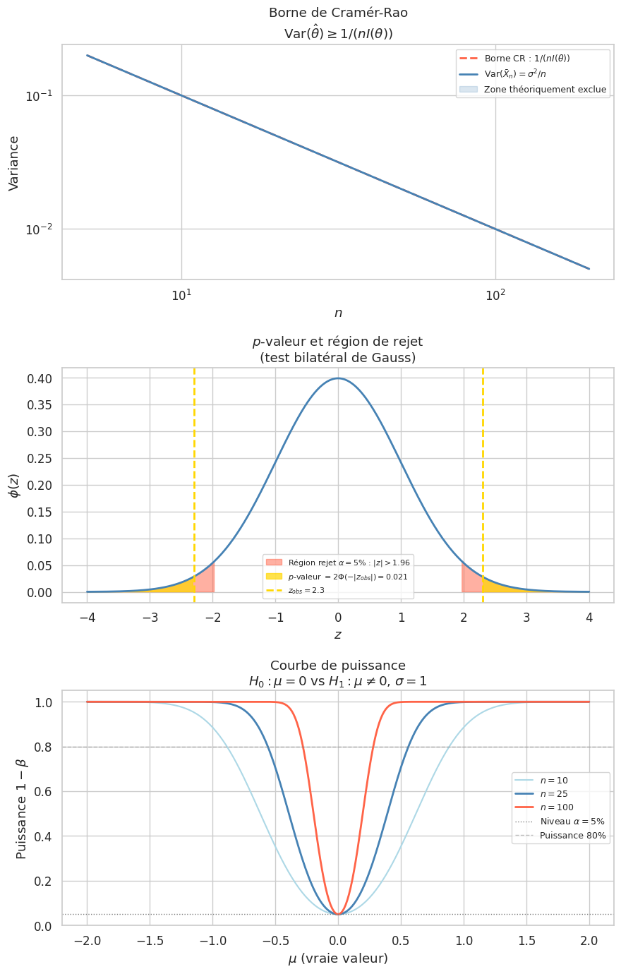
Théorème 85 (Borne de Cramér-Rao)

Pour tout estimateur sans biais \(\hat{\theta}\) de \(\theta\) :

\[\text{Var}(\hat{\theta}) \geq \frac{1}{nI(\theta)}\]

Un estimateur atteignant cette borne est dit efficace.

Proof. Par l’inégalité de Cauchy-Schwarz appliquée à \(\text{Cov}\!\left(\hat{\theta}, \frac{\partial}{\partial\theta}\ln L(\theta)\right)\) où \(L(\theta) = \prod f_\theta(X_i)\) :

\[\text{Var}(\hat{\theta}) \cdot \text{Var}\!\left(\frac{\partial \ln L}{\partial\theta}\right) \geq \left[\text{Cov}\!\left(\hat{\theta}, \frac{\partial \ln L}{\partial\theta}\right)\right]^2\]

En dérivant \(\mathbb{E}_\theta[\hat{\theta}] = \theta\) sous le signe intégral (hypothèse de régularité) :

\[\text{Cov}\!\left(\hat{\theta}, \frac{\partial \ln L}{\partial\theta}\right) = 1\]

Et \(\text{Var}\!\left(\frac{\partial \ln L}{\partial\theta}\right) = nI(\theta)\), d’où \(\text{Var}(\hat{\theta}) \geq 1/(nI(\theta))\).

Exemple 161

Modèle gaussien \(\mathcal{N}(\theta, \sigma^2)\) (\(\sigma^2\) connu) : \(\ln f_\theta(x) = -\frac{(x-\theta)^2}{2\sigma^2} + \text{cte}\). \(\frac{\partial \ln f}{\partial\theta} = \frac{x-\theta}{\sigma^2}\). \(I(\theta) = \mathbb{E}\!\left[\left(\frac{X-\theta}{\sigma^2}\right)^2\right] = \frac{1}{\sigma^2}\).

Borne CR : \(\text{Var}(\hat{\theta}) \geq \sigma^2/n\). L’EMV \(\bar{X}_n\) vérifie \(\text{Var}(\bar{X}_n) = \sigma^2/n\) : il est efficace.

Méthode du maximum de vraisemblance

Définition 300 (Vraisemblance et EMV)

La fonction de vraisemblance pour l’observation \((x_1, \ldots, x_n)\) est

\[L(\theta) = \prod_{i=1}^n f_\theta(x_i)\]

La log-vraisemblance est \(\ell(\theta) = \sum_{i=1}^n \ln f_\theta(x_i)\).

L”estimateur du maximum de vraisemblance (EMV) est \(\hat{\theta}_{MV} = \arg\max_\theta L(\theta)\).

Remarque 143

L’EMV est en général : (1) convergent \(\hat{\theta}_{MV} \xrightarrow{\mathbb{P}} \theta\), (2) asymptotiquement normal \(\sqrt{n}(\hat{\theta}_{MV} - \theta) \xrightarrow{\mathcal{L}} \mathcal{N}(0, 1/I(\theta))\), (3) asymptotiquement efficace (atteint la borne CR asymptotiquement). C’est la méthode d’estimation la plus utilisée en pratique.

Exemple 162

Loi normale \(\mathcal{N}(\mu, \sigma^2)\), les deux paramètres inconnus :

\[\ell(\mu, \sigma^2) = -\frac{n}{2}\ln(2\pi\sigma^2) - \frac{1}{2\sigma^2}\sum(x_i - \mu)^2\]

\(\partial\ell/\partial\mu = 0 \implies \hat{\mu}_{MV} = \bar{x}\) \(\partial\ell/\partial\sigma^2 = 0 \implies \hat{\sigma}^2_{MV} = \frac{1}{n}\sum(x_i - \bar{x})^2 = S_n^2\) (biaisé, mais convergent).

Exemple 163

Loi de Bernoulli \(\mathcal{B}(p)\) : \(L(p) = p^{\sum x_i}(1-p)^{n-\sum x_i}\). \(\ell'(p) = \frac{\sum x_i}{p} - \frac{n - \sum x_i}{1-p} = 0 \implies \hat{p}_{MV} = \bar{x}\) (proportion empirique).

Intervalles de confiance

Définition 301 (Intervalle de confiance)

Un intervalle de confiance (IC) au niveau \(1 - \alpha\) pour \(\theta\) est un intervalle aléatoire \([T_1, T_2]\) tel que

\[\mathbb{P}_\theta(\theta \in [T_1, T_2]) \geq 1 - \alpha \quad \forall \theta \in \Theta\]

Remarque 144

Interprétation fréquentiste : si on répète l’expérience beaucoup de fois, environ \(100(1-\alpha)\%\) des intervalles construits contiennent \(\theta\). Ce n’est pas «\(\theta\) est dans l’intervalle avec probabilité \(95\%\)» — \(\theta\) est fixe.

Proposition 344 (IC pour \(\mu\) avec \(\sigma\) connu)

Si \(X_1, \ldots, X_n\) i.i.d. \(\mathcal{N}(\mu, \sigma^2)\) :

\[\left[\bar{X}_n - z_{\alpha/2}\frac{\sigma}{\sqrt{n}}, \; \bar{X}_n + z_{\alpha/2}\frac{\sigma}{\sqrt{n}}\right]\]

est un IC de niveau exact \(1 - \alpha\), où \(z_{\alpha/2} = \Phi^{-1}(1 - \alpha/2)\). Pour \(\alpha = 0{,}05\) : \(z_{0{,}025} = 1{,}96\).

Proof. \(Z = \frac{\bar{X}_n - \mu}{\sigma/\sqrt{n}} \sim \mathcal{N}(0,1)\) exactement. \(\mathbb{P}(-z_{\alpha/2} \leq Z \leq z_{\alpha/2}) = 1-\alpha\). En isolant \(\mu\) : \(\mathbb{P}(\bar{X}_n - z_{\alpha/2}\sigma/\sqrt{n} \leq \mu \leq \bar{X}_n + z_{\alpha/2}\sigma/\sqrt{n}) = 1-\alpha\).

Définition 302 (Loi de Student)

Si \(Z \sim \mathcal{N}(0,1)\) et \(V \sim \chi^2(n)\) sont indépendantes, alors \(T = Z/\sqrt{V/n}\) suit la loi de Student \(t(n)\). Sa densité est

\[f_n(t) = \frac{\Gamma((n+1)/2)}{\sqrt{n\pi}\,\Gamma(n/2)}\left(1+\frac{t^2}{n}\right)^{-(n+1)/2}\]

Pour \(n \to \infty\) : \(t(n) \to \mathcal{N}(0,1)\).

Proposition 345 (IC pour \(\mu\) avec \(\sigma\) inconnu)

\[\left[\bar{X}_n - t_{\alpha/2, n-1}\frac{S_n'}{\sqrt{n}}, \; \bar{X}_n + t_{\alpha/2, n-1}\frac{S_n'}{\sqrt{n}}\right]\]

est un IC de niveau exact \(1-\alpha\), où \(t_{\alpha/2, n-1}\) est le quantile de \(t(n-1)\).

Proof. Pour un échantillon gaussien, \(\bar{X}_n\) et \(S_n'^2\) sont indépendantes (théorème de Fisher-Cochran) et \((n-1)S_n'^2/\sigma^2 \sim \chi^2(n-1)\). Donc

\[T = \frac{\bar{X}_n - \mu}{S_n'/\sqrt{n}} = \frac{(\bar{X}_n - \mu)/(\sigma/\sqrt{n})}{\sqrt{(n-1)S_n'^2/\sigma^2/(n-1)}} \sim t(n-1)\]

Proposition 346 (IC pour une proportion (grand échantillon))

Si \(X_1, \ldots, X_n\) i.i.d. \(\mathcal{B}(p)\) et \(n\) grand :

\[\hat{p} \pm z_{\alpha/2}\sqrt{\frac{\hat{p}(1-\hat{p})}{n}}\]

où \(\hat{p} = \bar{X}_n\). Par le TCL : \((\hat{p} - p)/\sqrt{p(1-p)/n} \xrightarrow{\mathcal{L}} \mathcal{N}(0,1)\).

Tests d’hypothèses

Définition 303 (Test statistique)

Un test confronte deux hypothèses :

• \(H_0\) : l”hypothèse nulle (statu quo)

• \(H_1\) : l”hypothèse alternative

Un test est une règle de décision basée sur l’échantillon : on rejette \(H_0\) si la statistique de test tombe dans la région de rejet \(W\).

Définition 304 (Erreurs et puissance)

	\(H_0\) vraie	\(H_1\) vraie
Accepter \(H_0\)	Correct	Erreur type II (\(\beta\))
Rejeter \(H_0\)	Erreur type I (\(\alpha\))	Correct (puissance)

• Risque de 1re espèce : \(\alpha = \mathbb{P}_{H_0}(\text{rejeter } H_0)\) (faux positif)

• Risque de 2e espèce : \(\beta = \mathbb{P}_{H_1}(\text{accepter } H_0)\) (faux négatif)

• Puissance : \(1 - \beta = \mathbb{P}_{H_1}(\text{rejeter } H_0)\)

Un test est de niveau \(\alpha\) si \(\sup_{\theta \in H_0} \mathbb{P}_\theta(\text{rejeter}) \leq \alpha\).

Exemple 164

Test de Gauss \(H_0 : \mu = \mu_0\) contre \(H_1 : \mu \neq \mu_0\), \(\sigma\) connu.

Statistique : \(Z = \frac{\bar{X}_n - \mu_0}{\sigma/\sqrt{n}}\). Sous \(H_0\) : \(Z \sim \mathcal{N}(0,1)\). Région de rejet : \(|Z| > z_{\alpha/2}\).

Décision : rejeter \(H_0\) si \(|\bar{X}_n - \mu_0| > z_{\alpha/2} \cdot \sigma/\sqrt{n}\).

Définition 305 (\(p\)-valeur)

La \(p\)-valeur est la probabilité, sous \(H_0\), d’observer un résultat au moins aussi extrême que celui observé :

\[p = \mathbb{P}_{H_0}(|Z| \geq |z_{\text{obs}}|) = 2(1 - \Phi(|z_{\text{obs}}|))\]

On rejette \(H_0\) au niveau \(\alpha\) si et seulement si \(p \leq \alpha\).

La \(p\)-valeur est le plus petit niveau \(\alpha\) auquel on rejetterait \(H_0\).

Théorème 86 (Test du \(\chi^2\) de Pearson)

Soit \(n\) observations classées en \(k\) catégories, effectifs observés \(O_i\) et théoriques \(E_i = np_i\) sous \(H_0\). La statistique

\[\chi^2 = \sum_{i=1}^k \frac{(O_i - E_i)^2}{E_i}\]

suit approximativement \(\chi^2(k-1-r)\) sous \(H_0\) (\(r\) = nombre de paramètres estimés). On rejette \(H_0\) si \(\chi^2 > \chi^2_{\alpha, k-1-r}\).

Show code cell source

Hide code cell source

fig, axes = plt.subplots(3, 1, figsize=(9, 14))

# 1. Borne de Cramer-Rao : variance de l'EMV vs borne
ax = axes[0]
ns = np.arange(5, 200)
# N(mu, sigma^2=1) : I(mu) = 1, borne CR = 1/n
cr_bound = 1 / ns
# Variance simulee de Xbar
var_xbar = 1 / ns  # exactement egal a la borne
ax.plot(ns, cr_bound, 'tomato', lw=2, linestyle='--', label='Borne CR : $1/(nI(\\theta))$')
ax.plot(ns, var_xbar, 'steelblue', lw=2, label='$\\text{Var}(\\bar{X}_n) = \\sigma^2/n$')
ax.fill_between(ns, cr_bound, var_xbar, alpha=0.2, color='steelblue',
                label='Zone théoriquement exclue')
ax.set_xlabel('$n$'); ax.set_ylabel('Variance')
ax.set_title('Borne de Cramér-Rao\n$\\text{Var}(\\hat{\\theta}) \\geq 1/(nI(\\theta))$')
ax.legend(fontsize=9); ax.set_xscale('log'); ax.set_yscale('log')

# 2. p-valeur : illustration
ax = axes[1]
z = np.linspace(-4, 4, 400)
phi = stats.norm.pdf(z)
ax.plot(z, phi, 'steelblue', lw=2)
z_obs = 2.3  # valeur observee
# Zone de rejet
alpha = 0.05
z_crit = stats.norm.ppf(1 - alpha/2)
ax.fill_between(z, phi, where=np.abs(z) > z_crit, color='tomato', alpha=0.5,
                label=f'Région rejet $\\alpha=5\\%$ : $|z|>{z_crit:.2f}$')
# p-valeur
ax.fill_between(z, phi, where=np.abs(z) > np.abs(z_obs), color='gold', alpha=0.7,
                label=f'$p$-valeur $= 2\\Phi(-|z_{{obs}}|) = {2*stats.norm.sf(np.abs(z_obs)):.3f}$')
ax.axvline(z_obs, color='gold', lw=2, linestyle='--', label=f'$z_{{obs}}={z_obs}$')
ax.axvline(-z_obs, color='gold', lw=2, linestyle='--')
ax.set_xlabel('$z$'); ax.set_ylabel('$\\phi(z)$')
ax.set_title('$p$-valeur et région de rejet\n(test bilatéral de Gauss)')
ax.legend(fontsize=8)

# 3. Puissance du test en fonction de mu
ax = axes[2]
mu_0 = 0; sigma = 1; n_pw = 25
z_crit_pw = stats.norm.ppf(1 - 0.05/2)
mu_alt = np.linspace(-2, 2, 300)
# Puissance : P(|Z| > z_crit | mu = mu_alt)
z_eff = np.abs(mu_alt) * np.sqrt(n_pw) / sigma
power = stats.norm.cdf(-z_crit_pw + np.abs(mu_alt)*np.sqrt(n_pw)) + \
        stats.norm.sf(z_crit_pw + np.abs(mu_alt)*np.sqrt(n_pw))
# Pour differentes tailles n
for n_p, color, lw in [(10, 'lightblue', 1.5), (25, 'steelblue', 2), (100, 'tomato', 2)]:
    pw = stats.norm.cdf(-z_crit_pw + np.abs(mu_alt)*np.sqrt(n_p)) + \
         stats.norm.sf(z_crit_pw + np.abs(mu_alt)*np.sqrt(n_p))
    ax.plot(mu_alt, pw, color=color, lw=lw, label=f'$n={n_p}$')
ax.axhline(0.05, color='gray', lw=1, linestyle=':', label='Niveau $\\alpha=5\\%$')
ax.axhline(0.8, color='gray', lw=1, linestyle='--', alpha=0.5, label='Puissance 80%')
ax.set_xlabel('$\\mu$ (vraie valeur)'); ax.set_ylabel('Puissance $1-\\beta$')
ax.set_title('Courbe de puissance\n$H_0:\\mu=0$ vs $H_1:\\mu\\neq 0$, $\\sigma=1$')
ax.legend(fontsize=9); ax.set_ylim(0, 1.05)

plt.tight_layout()
plt.show()

Résumé

Concept	Propriété clé
Estimateur sans biais	\(\mathbb{E}[\hat{\theta}] = \theta\)
EQM	\(\text{Var}(\hat{\theta}) + b(\hat{\theta})^2\)
Convergent	\(\hat{\theta}_n \xrightarrow{\mathbb{P}} \theta\)
Info. de Fisher	\(I(\theta) = \mathbb{E}[(\partial_\theta \ln f_\theta)^2]\)
Cramér-Rao	\(\text{Var}(\hat{\theta}) \geq 1/(nI(\theta))\)
EMV	\(\arg\max L(\theta)\), asymptotiquement efficace
IC pour \(\mu\) (\(\sigma\) connu)	\(\bar{X} \pm z_{\alpha/2}\sigma/\sqrt{n}\), niveau exact
IC pour \(\mu\) (\(\sigma\) inconnu)	\(\bar{X} \pm t_{\alpha/2,n-1}S'/\sqrt{n}\), loi de Student
IC pour \(p\)	\(\hat{p} \pm z_{\alpha/2}\sqrt{\hat{p}(1-\hat{p})/n}\)
\(p\)-valeur	Rejeter \(H_0\) si \(p \leq \alpha\)
Test \(\chi^2\)	\(\sum(O_i-E_i)^2/E_i \sim \chi^2(k-1-r)\)