Probabilités discrètes

La théorie des probabilités n’est au fond que le bon sens réduit au calcul.

Pierre-Simon de Laplace

Introduction

Les probabilités formalisent la notion d”incertitude et de hasard. Là où l’analyse étudie des quantités déterministes, la théorie des probabilités étudie des phénomènes dont l’issue n’est pas certaine. Ce chapitre pose les fondements : espaces probabilisés, variables aléatoires discrètes, espérance, variance, et les lois classiques.

Show code cell source

Hide code cell source

import numpy as np
import matplotlib.pyplot as plt
import seaborn as sns
from scipy import stats

sns.set_theme(style="whitegrid", palette="muted", font_scale=1.1)

fig, axes = plt.subplots(3, 1, figsize=(9, 14))

# 1. Illustration du paradoxe de Bayes : test médical
ax = axes[0]
prev = np.linspace(0.001, 0.3, 300)
sens, spec = 0.99, 0.95
ppv = (sens * prev) / (sens * prev + (1 - spec) * (1 - prev))
ax.plot(prev * 100, ppv * 100, 'steelblue', lw=2.5)
ax.axvline(1, color='tomato', linestyle='--', lw=1.5, label='Prévalence 1%')
ppv_1 = (sens * 0.01) / (sens * 0.01 + (1 - spec) * 0.99)
ax.scatter([1], [ppv_1*100], color='tomato', s=100, zorder=5)
ax.annotate(f'$\\mathbb{{P}}(M|+) \\approx {ppv_1*100:.1f}\\%$', xy=(1, ppv_1*100),
            xytext=(5, ppv_1*100 - 8), fontsize=9,
            arrowprops=dict(arrowstyle='->', color='tomato'))
ax.set_xlabel('Prévalence (%)')
ax.set_ylabel('Valeur prédictive positive (%)')
ax.set_title('Paradoxe de Bayes\n(sensibilité 99%, spécificité 95%)')
ax.legend()

# 2. Lois discrètes classiques
ax = axes[1]
x_b = np.arange(0, 21)
ax.bar(x_b, stats.binom.pmf(x_b, 20, 0.5), alpha=0.7, color='steelblue',
       label='$\\mathcal{B}(20, 0.5)$', width=0.4, align='center')
ax.bar(x_b + 0.4, stats.binom.pmf(x_b, 20, 0.3), alpha=0.7, color='tomato',
       label='$\\mathcal{B}(20, 0.3)$', width=0.4, align='center')
ax2 = ax.twinx()
x_p = np.arange(0, 21)
ax2.plot(x_p, stats.poisson.pmf(x_p, 5), 'gold', lw=2, marker='o', ms=4,
         label='$\\mathcal{P}(5)$')
ax.set_xlabel('$k$'); ax.set_ylabel('$\\mathbb{P}(X=k)$')
ax.set_title('Lois discrètes classiques')
lines1, labels1 = ax.get_legend_handles_labels()
lines2, labels2 = ax2.get_legend_handles_labels()
ax.legend(lines1 + lines2, labels1 + labels2, fontsize=9)

# 3. Fonction génératrice : G(s) pour lois classiques
ax = axes[2]
s = np.linspace(0, 1, 200)
# B(10, 0.4) : G(s) = (0.6 + 0.4s)^10
G_binom = (0.6 + 0.4*s)**10
# Poisson(3) : G(s) = exp(3(s-1))
G_pois = np.exp(3*(s-1))
# Geometrique(0.4) : G(s) = 0.4s/(1-0.6s)
G_geom = 0.4*s / (1 - 0.6*s)
ax.plot(s, G_binom, 'steelblue', lw=2, label='$\\mathcal{B}(10,0.4)$: $(0.6+0.4s)^{10}$')
ax.plot(s, G_pois, 'tomato', lw=2, label='$\\mathcal{P}(3)$: $e^{3(s-1)}$')
ax.plot(s, G_geom, 'gold', lw=2, label='$\\mathcal{G}(0.4)$: $\\frac{0.4s}{1-0.6s}$')
ax.axvline(1, color='gray', lw=0.8, linestyle='--')
ax.scatter([1, 1, 1], [1, 1, 1], color=['steelblue','tomato','gold'], s=80, zorder=5)
ax.set_xlabel('$s$'); ax.set_ylabel('$G_X(s) = \\mathbb{E}[s^X]$')
ax.set_title('Fonctions génératrices\n$G_X(1)=1$, $G_X\'(1)=\\mathbb{E}[X]$')
ax.legend(fontsize=8); ax.set_ylim(0, 1.1)

plt.tight_layout()
plt.show()

Espaces probabilisés

Définition 272 (Tribu (\(\sigma\)-algèbre))

Soit \(\Omega\) un ensemble (l”univers). Une tribu sur \(\Omega\) est une famille \(\mathcal{A} \subset \mathcal{P}(\Omega)\) vérifiant :

1. \(\Omega \in \mathcal{A}\)

2. \(A \in \mathcal{A} \implies \bar{A} = \Omega \setminus A \in \mathcal{A}\)

3. \((A_n)_{n \geq 1} \subset \mathcal{A} \implies \bigcup_{n=1}^\infty A_n \in \mathcal{A}\)

Remarque 138

Par De Morgan, \(\mathcal{A}\) est stable par intersection dénombrable. Les éléments de \(\mathcal{A}\) sont les événements. En cas discret, on prend \(\mathcal{A} = \mathcal{P}(\Omega)\).

Définition 273 (Probabilité)

Une probabilité sur \((\Omega, \mathcal{A})\) est \(\mathbb{P} : \mathcal{A} \to [0, 1]\) vérifiant :

1. \(\mathbb{P}(\Omega) = 1\)

2. \(\sigma\)-additivité : pour \((A_n)\) deux à deux disjoints : \(\mathbb{P}\bigl(\bigcup_{n=1}^\infty A_n\bigr) = \sum_{n=1}^\infty \mathbb{P}(A_n)\)

Le triplet \((\Omega, \mathcal{A}, \mathbb{P})\) est un espace probabilisé.

Proposition 331 (Propriétés fondamentales)

• \(\mathbb{P}(\bar{A}) = 1 - \mathbb{P}(A)\)

• \(\mathbb{P}(\varnothing) = 0\)

• \(A \subset B \implies \mathbb{P}(A) \leq \mathbb{P}(B)\)

• \(\mathbb{P}(A \cup B) = \mathbb{P}(A) + \mathbb{P}(B) - \mathbb{P}(A \cap B)\)

• Continuité croissante : \(A_n \nearrow A \implies \mathbb{P}(A_n) \to \mathbb{P}(A)\)

• Continuité décroissante : \(A_n \searrow A \implies \mathbb{P}(A_n) \to \mathbb{P}(A)\)

Proof. Complémentaire : \(1 = \mathbb{P}(\Omega) = \mathbb{P}(A \sqcup \bar{A}) = \mathbb{P}(A) + \mathbb{P}(\bar{A})\).

Inclusion-exclusion : \(A \cup B = A \sqcup (B \setminus A)\) et \(\mathbb{P}(B \setminus A) = \mathbb{P}(B) - \mathbb{P}(A \cap B)\).

Continuité croissante : \(A_n \nearrow A \implies A = A_1 \sqcup (A_2 \setminus A_1) \sqcup \cdots\), et \(\mathbb{P}(A) = \mathbb{P}(A_1) + \sum_{k \geq 1} \mathbb{P}(A_{k+1} \setminus A_k) = \lim_n \mathbb{P}(A_n)\).

Probabilités conditionnelles et indépendance

Définition 274 (Probabilité conditionnelle)

Soit \(B\) un événement avec \(\mathbb{P}(B) > 0\). La probabilité de \(A\) sachant \(B\) est

\[\mathbb{P}(A \mid B) = \frac{\mathbb{P}(A \cap B)}{\mathbb{P}(B)}\]

Théorème 72 (Formule des probabilités totales)

Soit \((B_i)_{i \in I}\) un système complet d’événements (deux à deux disjoints, \(\bigcup B_i = \Omega\), \(\mathbb{P}(B_i) > 0\)). Pour tout \(A\) :

\[\mathbb{P}(A) = \sum_{i \in I} \mathbb{P}(A \mid B_i) \, \mathbb{P}(B_i)\]

Proof. \(A = \bigsqcup_i (A \cap B_i)\), donc \(\mathbb{P}(A) = \sum_i \mathbb{P}(A \cap B_i) = \sum_i \mathbb{P}(A \mid B_i)\mathbb{P}(B_i)\).

Théorème 73 (Formule de Bayes)

Sous les mêmes hypothèses :

\[\mathbb{P}(B_j \mid A) = \frac{\mathbb{P}(A \mid B_j) \, \mathbb{P}(B_j)}{\displaystyle\sum_{i} \mathbb{P}(A \mid B_i) \, \mathbb{P}(B_i)}\]

Proof. \(\mathbb{P}(B_j \mid A) = \frac{\mathbb{P}(A \cap B_j)}{\mathbb{P}(A)} = \frac{\mathbb{P}(A \mid B_j)\mathbb{P}(B_j)}{\mathbb{P}(A)}\). On remplace \(\mathbb{P}(A)\) par la formule des probabilités totales.

Exemple 152

Test médical. Prévalence \(\mathbb{P}(M) = 1\%\). Sensibilité \(\mathbb{P}(+ \mid M) = 99\%\). Spécificité \(\mathbb{P}(- \mid \bar{M}) = 95\%\), donc \(\mathbb{P}(+ \mid \bar{M}) = 5\%\).

\[\mathbb{P}(M \mid +) = \frac{0{,}99 \times 0{,}01}{0{,}99 \times 0{,}01 + 0{,}05 \times 0{,}99} = \frac{0{,}0099}{0{,}0594} \approx 16{,}7\%\]

Un test positif ne donne que \(\approx 17\%\) de chances d’être malade — résultat contre-intuitif, dû à la faible prévalence.

Définition 275 (Indépendance)

Deux événements \(A, B\) sont indépendants si \(\mathbb{P}(A \cap B) = \mathbb{P}(A) \cdot \mathbb{P}(B)\).

Une famille \((A_i)_{i \in I}\) est mutuellement indépendante si pour toute partie finie \(J \subset I\) :

\[\mathbb{P}\Bigl(\bigcap_{j \in J} A_j\Bigr) = \prod_{j \in J} \mathbb{P}(A_j)\]

Remarque 139

L’indépendance deux à deux n’implique pas l’indépendance mutuelle. Contre-exemple (Bernstein) : deux dés, \(A = \{\text{1er pair}\}\), \(B = \{\text{2e pair}\}\), \(C = \{\text{somme paire}\}\).

Variables aléatoires discrètes

Définition 276 (Variable aléatoire discrète)

Une variable aléatoire discrète est une application \(X : \Omega \to E\) (avec \(E\) dénombrable) mesurable : \(\{X = x\} \in \mathcal{A}\) pour tout \(x \in E\).

La loi de \(X\) est la famille \((\mathbb{P}(X = x))_{x \in E}\), avec \(\sum_{x \in E} \mathbb{P}(X = x) = 1\).

Lois discrètes classiques

Définition 277 (Lois discrètes fondamentales)

Bernoulli \(\mathcal{B}(p)\) : \(X \in \{0,1\}\), \(\mathbb{P}(X=1) = p\), \(\mathbb{P}(X=0) = 1-p\).

Binomiale \(\mathcal{B}(n,p)\) : \(X \in \{0,\ldots,n\}\), \(\mathbb{P}(X=k) = \binom{n}{k}p^k(1-p)^{n-k}\). Modélise le nombre de succès dans \(n\) épreuves de Bernoulli indépendantes.

Poisson \(\mathcal{P}(\lambda)\) : \(X \in \mathbb{N}\), \(\mathbb{P}(X=k) = e^{-\lambda}\frac{\lambda^k}{k!}\), \(\lambda > 0\). Modélise le nombre d’occurrences d’un événement rare.

Géométrique \(\mathcal{G}(p)\) : \(X \in \mathbb{N}^*\), \(\mathbb{P}(X=k) = (1-p)^{k-1}p\). Modélise le rang du premier succès.

Proposition 332 (Vérification \(\sum \mathbb{P}(X=k) = 1\))

• Binomiale : \(\sum_{k=0}^n \binom{n}{k}p^k q^{n-k} = (p+q)^n = 1\).

• Poisson : \(\sum_{k=0}^\infty e^{-\lambda}\frac{\lambda^k}{k!} = e^{-\lambda} e^\lambda = 1\).

• Géométrique : \(\sum_{k=1}^\infty (1-p)^{k-1}p = p \cdot \frac{1}{1-(1-p)} = 1\).

Proposition 333 (Absence de mémoire de la loi géométrique)

La loi géométrique est l’unique loi discrète vérifiant :

\[\mathbb{P}(X > m + n \mid X > m) = \mathbb{P}(X > n)\]

Proof. \(\mathbb{P}(X > k) = (1-p)^k\). Donc \(\mathbb{P}(X > m+n \mid X > m) = \frac{(1-p)^{m+n}}{(1-p)^m} = (1-p)^n = \mathbb{P}(X>n)\).

Unicité : Si \(g(t) = \mathbb{P}(X > t)\) vérifie \(g(m+n) = g(m)g(n)\) avec \(g\) décroissante et \(g(0) = 1\), alors par récurrence \(g(k) = g(1)^k\), ce qui donne la loi géométrique avec \(p = 1 - g(1)\).

Espérance

Définition 278 (Espérance)

L”espérance de \(X\) est (si la somme converge absolument) :

\[\mathbb{E}[X] = \sum_{x \in X(\Omega)} x \cdot \mathbb{P}(X = x)\]

Théorème 74 (Formule de transfert)

Si \(g : E \to \mathbb{R}\), alors \(\mathbb{E}[g(X)] = \sum_{x \in X(\Omega)} g(x) \cdot \mathbb{P}(X = x)\).

Proposition 334 (Propriétés de l’espérance)

• Linéarité : \(\mathbb{E}[\alpha X + \beta Y] = \alpha \mathbb{E}[X] + \beta \mathbb{E}[Y]\) (toujours, sans hypothèse d’indépendance)

• Positivité : \(X \geq 0 \implies \mathbb{E}[X] \geq 0\)

• Monotonie : \(X \leq Y \implies \mathbb{E}[X] \leq \mathbb{E}[Y]\)

• Produit si indépendantes : \(X \perp Y \implies \mathbb{E}[XY] = \mathbb{E}[X]\mathbb{E}[Y]\)

Proposition 335 (Espérances des lois classiques)

Loi	\(\mathbb{E}[X]\)	\(\text{Var}(X)\)
\(\mathcal{B}(p)\)	\(p\)	\(p(1-p)\)
\(\mathcal{B}(n,p)\)	\(np\)	\(np(1-p)\)
\(\mathcal{P}(\lambda)\)	\(\lambda\)	\(\lambda\)
\(\mathcal{G}(p)\)	\(1/p\)	\((1-p)/p^2\)
\(\mathcal{U}(\{1,\ldots,n\})\)	\((n+1)/2\)	\((n^2-1)/12\)

Proof. Binomiale : Écrire \(X = X_1 + \cdots + X_n\) avec \(X_i \sim \mathcal{B}(p)\) i.i.d. Par linéarité : \(\mathbb{E}[X] = n\mathbb{E}[X_1] = np\). Pour la variance (indépendance) : \(\text{Var}(X) = n\text{Var}(X_1) = np(1-p)\).

Poisson : \(\mathbb{E}[X] = \sum_{k=1}^\infty k e^{-\lambda}\frac{\lambda^k}{k!} = \lambda e^{-\lambda} \sum_{k=1}^\infty \frac{\lambda^{k-1}}{(k-1)!} = \lambda e^{-\lambda} e^\lambda = \lambda\).

\(\mathbb{E}[X(X-1)] = \lambda^2\) (calcul analogue), donc \(\text{Var}(X) = \mathbb{E}[X^2] - \lambda^2 = \mathbb{E}[X(X-1)] + \mathbb{E}[X] - \lambda^2 = \lambda^2 + \lambda - \lambda^2 = \lambda\).

Géométrique : \(\mathbb{E}[X] = \sum_{k=1}^\infty k(1-p)^{k-1}p = p \cdot \frac{d}{dq}\sum_{k=1}^\infty q^k\big|_{q=1-p} = p \cdot \frac{1}{p^2} = \frac{1}{p}\).

Variance et inégalités

Définition 279 (Variance)

\[\text{Var}(X) = \mathbb{E}[(X - \mathbb{E}[X])^2] = \mathbb{E}[X^2] - (\mathbb{E}[X])^2\]

Lӎcart-type est \(\sigma(X) = \sqrt{\text{Var}(X)}\).

Proof. Formule de König-Huygens : \(\text{Var}(X) = \mathbb{E}[(X-\mu)^2] = \mathbb{E}[X^2 - 2\mu X + \mu^2] = \mathbb{E}[X^2] - 2\mu^2 + \mu^2 = \mathbb{E}[X^2] - \mu^2\).

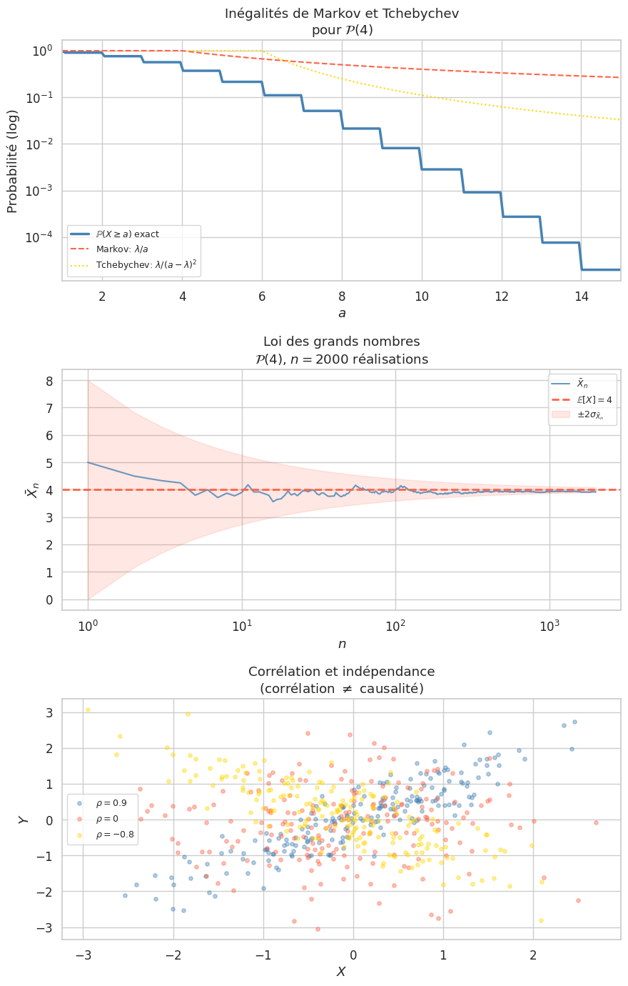
Théorème 75 (Inégalité de Markov)

Si \(X \geq 0\), alors pour tout \(a > 0\) :

\[\mathbb{P}(X \geq a) \leq \frac{\mathbb{E}[X]}{a}\]

Proof. \(\mathbb{E}[X] = \sum_x x \mathbb{P}(X=x) \geq \sum_{x \geq a} x \mathbb{P}(X=x) \geq a \sum_{x \geq a} \mathbb{P}(X=x) = a\mathbb{P}(X \geq a)\).

Théorème 76 (Inégalité de Bienaymé-Tchebychev)

\[\mathbb{P}(|X - \mathbb{E}[X]| \geq a) \leq \frac{\text{Var}(X)}{a^2}\]

Proof. Appliquer Markov à \(Y = (X - \mathbb{E}[X])^2 \geq 0\) : \(\mathbb{P}(Y \geq a^2) \leq \mathbb{E}[Y]/a^2 = \text{Var}(X)/a^2\).

Fonctions génératrices

Définition 280 (Fonction génératrice)

Soit \(X\) à valeurs dans \(\mathbb{N}\). La fonction génératrice est

\[G_X(s) = \mathbb{E}[s^X] = \sum_{k=0}^\infty \mathbb{P}(X = k) s^k, \quad |s| \leq 1\]

Proposition 336 (Propriétés)

• \(G_X(1) = 1\)

• \(G_X'(1) = \mathbb{E}[X]\)

• \(G_X''(1) = \mathbb{E}[X(X-1)]\), d’où \(\text{Var}(X) = G_X''(1) + G_X'(1) - (G_X'(1))^2\)

• \(G_X\) détermine la loi de \(X\) : \(\mathbb{P}(X = k) = G_X^{(k)}(0)/k!\)

• \(X, Y\) indépendantes \(\implies G_{X+Y} = G_X \cdot G_Y\)

Exemple 153

• \(\mathcal{B}(p)\) : \(G(s) = q + ps\)

• \(\mathcal{B}(n,p)\) : \(G(s) = (q + ps)^n\) (produit de \(n\) Bernoulli indépendantes)

• \(\mathcal{P}(\lambda)\) : \(G(s) = e^{\lambda(s-1)}\)

• \(\mathcal{G}(p)\) : \(G(s) = \frac{ps}{1 - qs}\) (pour \(|s| < 1/q\))

Somme de Poissons indépendantes : \(X \sim \mathcal{P}(\lambda)\), \(Y \sim \mathcal{P}(\mu)\) indépendantes. \(G_{X+Y}(s) = e^{\lambda(s-1)} \cdot e^{\mu(s-1)} = e^{(\lambda+\mu)(s-1)}\). Donc \(X + Y \sim \mathcal{P}(\lambda + \mu)\).

Couples de variables aléatoires

Définition 281 (Loi conjointe, marginales, indépendance)

La loi conjointe de \((X, Y)\) : \(\mathbb{P}(X=x, Y=y)\) pour tous \(x, y\).

Les lois marginales : \(\mathbb{P}(X=x) = \sum_y \mathbb{P}(X=x, Y=y)\).

\(X\) et \(Y\) sont indépendantes si \(\mathbb{P}(X=x, Y=y) = \mathbb{P}(X=x) \cdot \mathbb{P}(Y=y)\) pour tous \(x, y\).

Définition 282 (Covariance et corrélation)

\[\text{Cov}(X, Y) = \mathbb{E}[(X - \mathbb{E}X)(Y - \mathbb{E}Y)] = \mathbb{E}[XY] - \mathbb{E}[X]\mathbb{E}[Y]\]

Le coefficient de corrélation : \(\rho(X,Y) = \dfrac{\text{Cov}(X,Y)}{\sigma(X)\sigma(Y)} \in [-1, 1]\).

Proposition 337

• \(\text{Var}(X + Y) = \text{Var}(X) + \text{Var}(Y) + 2\text{Cov}(X,Y)\)

• \(X, Y\) indépendantes \(\implies \text{Cov}(X,Y) = 0\) (non corrélées)

• La réciproque est fausse en général

• \(|\rho(X,Y)| = 1 \iff Y = aX + b\) p.s. pour des constantes \(a, b\)

Proof. Indépendance \(\implies\) non-corrélation : \(\mathbb{E}[XY] = \sum_{x,y} xy \mathbb{P}(X=x)\mathbb{P}(Y=y) = \left(\sum_x x\mathbb{P}(X=x)\right)\left(\sum_y y\mathbb{P}(Y=y)\right) = \mathbb{E}[X]\mathbb{E}[Y]\).

\(|\rho|=1\) : \(\rho(X,Y)=1 \iff \text{Var}(Y - \frac{\sigma_Y}{\sigma_X}X) = 0 \iff Y = \frac{\sigma_Y}{\sigma_X}X + c\) p.s.

Show code cell source

Hide code cell source

fig, axes = plt.subplots(3, 1, figsize=(9, 14))

# 1. Illustration Markov et Tchebychev
ax = axes[0]
# Poisson(4) : P(X >= a) vs Markov et Tchebychev
lam = 4
a_vals = np.linspace(1, 15, 200)
x_max = 40
x_arr = np.arange(x_max+1)
pmf = stats.poisson.pmf(x_arr, lam)
px_ge_a = np.array([np.sum(pmf[int(np.ceil(a)):]) for a in a_vals])
markov = np.minimum(1, lam / a_vals)
tcheb = np.minimum(1, lam / (a_vals - lam)**2)
tcheb[a_vals <= lam] = 1

ax.semilogy(a_vals, px_ge_a, 'steelblue', lw=2.5, label='$\\mathbb{P}(X \\geq a)$ exact')
ax.semilogy(a_vals, markov, 'tomato', lw=1.5, linestyle='--', label='Markov: $\\lambda/a$')
ax.semilogy(a_vals[a_vals > lam+0.1], tcheb[a_vals > lam+0.1], 'gold', lw=1.5,
            linestyle=':', label='Tchebychev: $\\lambda/(a-\\lambda)^2$')
ax.set_xlabel('$a$'); ax.set_ylabel('Probabilité (log)')
ax.set_title('Inégalités de Markov et Tchebychev\npour $\\mathcal{P}(4)$')
ax.legend(fontsize=9); ax.set_xlim(1, 15)

# 2. Loi des grands nombres illustrée
ax = axes[1]
np.random.seed(42)
n_max = 2000
X = np.random.poisson(4, n_max)
means = np.cumsum(X) / np.arange(1, n_max+1)
ax.plot(range(1, n_max+1), means, 'steelblue', lw=1.5, alpha=0.8, label='$\\bar{X}_n$')
ax.axhline(4, color='tomato', lw=2, linestyle='--', label='$\\mathbb{E}[X]=4$')
# Bande Tchebychev 95%
n_arr = np.arange(1, n_max+1)
band = 2 * np.sqrt(4 / n_arr)  # 2 sigma_Xbar
ax.fill_between(n_arr, 4 - band, 4 + band, alpha=0.15, color='tomato', label='$\\pm 2\\sigma_{\\bar{X}_n}$')
ax.set_xlabel('$n$'); ax.set_ylabel('$\\bar{X}_n$')
ax.set_title('Loi des grands nombres\n$\\mathcal{P}(4)$, $n=2000$ réalisations')
ax.legend(fontsize=9); ax.set_xscale('log')

# 3. Covariance et corrélation
ax = axes[2]
np.random.seed(0)
# Trois nuages avec differentes correlations
for rho, color, label in [(0.9, 'steelblue', '$\\rho=0.9$'),
                           (0, 'tomato', '$\\rho=0$'),
                           (-0.8, 'gold', '$\\rho=-0.8$')]:
    cov = [[1, rho], [rho, 1]]
    pts = np.random.multivariate_normal([0, 0], cov, 200)
    ax.scatter(pts[:,0], pts[:,1], alpha=0.4, s=15, color=color, label=label)

ax.set_xlabel('$X$'); ax.set_ylabel('$Y$')
ax.set_title('Corrélation et indépendance\n(corrélation $\\neq$ causalité)')
ax.legend(fontsize=9)

plt.tight_layout()
plt.show()

Résumé

Concept	Formule / Propriété
Probabilité	\(\mathbb{P} : \mathcal{A} \to [0,1]\), \(\sigma\)-additive, \(\mathbb{P}(\Omega) = 1\)
Prob. conditionnelle	\(\mathbb{P}(A|B) = \mathbb{P}(A\cap B)/\mathbb{P}(B)\)
Bayes	\(\mathbb{P}(B_j|A) \propto \mathbb{P}(A|B_j)\mathbb{P}(B_j)\)
Espérance	\(\mathbb{E}[X] = \sum x\mathbb{P}(X=x)\), linéaire
Variance	\(\text{Var}(X) = \mathbb{E}[X^2] - \mathbb{E}[X]^2\)
Markov	\(\mathbb{P}(X \geq a) \leq \mathbb{E}[X]/a\)
Tchebychev	\(\mathbb{P}(|X-\mu| \geq a) \leq \sigma^2/a^2\)
Binomiale	\(\mathbb{E}=np\), \(\text{Var}=npq\), \(G=(q+ps)^n\)
Poisson	\(\mathbb{E}=\text{Var}=\lambda\), stable par somme
Géométrique	\(\mathbb{E}=1/p\), absence de mémoire
Indépendance	\(\mathbb{P}(X=x,Y=y)=\mathbb{P}(X=x)\mathbb{P}(Y=y)\)