Compléments sur ℂ#

Les nombres imaginaires sont une magnifique et merveilleuse ressource de l’esprit divin, presque un amphibie entre l’être et le non-être.

Gottfried Wilhelm Leibniz

Introduction#

Nous avons construit \(\mathbb{C}\) comme corps commutatif et établi ses propriétés fondamentales. Ce chapitre approfondit l’étude sous trois angles : algébrique (clôture algébrique, polynômes, Viète), géométrique (similitudes, lieux, cocyclicité, transformations de Möbius), et un aperçu analytique (logarithme complexe multi-valué, holomorphie).

Hide code cell source

import numpy as np
import matplotlib.pyplot as plt
import matplotlib.patches as patches
from matplotlib.patches import FancyArrowPatch

fig, axes = plt.subplots(3, 1, figsize=(9, 14))

# --- Racines 6-ièmes de l'unité ---
ax = axes[0]
n = 6
angles = [2*np.pi*k/n for k in range(n)]
roots = [np.exp(1j*t) for t in angles]
xs = [z.real for z in roots]
ys = [z.imag for z in roots]

circle = plt.Circle((0,0), 1, fill=False, color='steelblue', lw=1.5)
ax.add_patch(circle)
ax.scatter(xs, ys, s=80, color='tomato', zorder=5)
polygon = plt.Polygon(list(zip(xs, ys)), fill=False, edgecolor='tomato', lw=1, linestyle='--')
ax.add_patch(polygon)
for k, (x, y) in enumerate(zip(xs, ys)):
    ax.annotate(f'$\\omega^{k}$', (x, y), textcoords='offset points', xytext=(8*np.sign(x)+2, 8*np.sign(y)+2), fontsize=9)
ax.set_xlim(-1.4, 1.4); ax.set_ylim(-1.4, 1.4)
ax.set_aspect('equal'); ax.axhline(0, color='k', lw=0.5); ax.axvline(0, color='k', lw=0.5)
ax.set_title('Racines 6-ièmes de l\'unité', fontsize=11)
ax.set_xlabel('Re'); ax.set_ylabel('Im')

# --- Exponentielle complexe : lignes horizontales -> spirales ---
ax = axes[1]
# Re(z) = cst -> cercles ; Im(z) = cst -> rayons
for a in np.linspace(-1, 1, 5):
    t = np.linspace(0, 2*np.pi, 200)
    z = np.exp(a + 1j*t)
    ax.plot(z.real, z.imag, lw=1.5, alpha=0.7, label=f'Re={a:.1f}')
for b in np.linspace(0, np.pi, 5):
    r = np.linspace(0, 2, 100)
    z = np.exp(r + 1j*b)
    ax.plot(z.real, z.imag, lw=1, color='gray', alpha=0.5, linestyle='--')
ax.set_xlim(-8, 8); ax.set_ylim(-8, 8)
ax.set_aspect('equal'); ax.axhline(0, color='k', lw=0.5); ax.axvline(0, color='k', lw=0.5)
ax.set_title('Image de $e^{a+it}$ : cercles concentrés', fontsize=11)
ax.set_xlabel('Re'); ax.set_ylabel('Im')
ax.legend(fontsize=7, loc='upper left')

# --- Plan complexe : argument et module ---
ax = axes[2]
z0 = 2 + 1.5j
ax.annotate('', xy=(z0.real, z0.imag), xytext=(0, 0),
            arrowprops=dict(arrowstyle='->', color='tomato', lw=2))
ax.scatter([z0.real], [z0.imag], color='tomato', s=80, zorder=5)
ax.annotate(f'$z_0 = {z0.real}+{z0.imag}i$\n$|z_0|={abs(z0):.2f}$\n$\\arg(z_0)={np.angle(z0, deg=True):.1f}°$',
            (z0.real, z0.imag), xytext=(0.3, 1.7), fontsize=9)
theta = np.linspace(0, np.angle(z0), 100)
r_arc = 0.5
ax.plot(r_arc*np.cos(theta), r_arc*np.sin(theta), 'b-', lw=1.5)
ax.text(0.6*np.cos(np.angle(z0)/2), 0.6*np.sin(np.angle(z0)/2), r'$\arg(z_0)$', fontsize=9, color='b')
ax.plot([0, abs(z0)*np.cos(np.angle(z0))], [0, 0], 'g--', lw=1)
ax.plot([abs(z0)*np.cos(np.angle(z0)), z0.real], [0, z0.imag], 'g--', lw=1)
ax.text(abs(z0)/2, -0.2, f'$|z_0|\\cos\\theta$', fontsize=8, color='g')
ax.set_xlim(-0.5, 3.5); ax.set_ylim(-0.5, 2.5)
ax.set_aspect('equal'); ax.axhline(0, color='k', lw=0.5); ax.axvline(0, color='k', lw=0.5)
ax.set_title('Module et argument', fontsize=11)
ax.set_xlabel('Re'); ax.set_ylabel('Im')

plt.suptitle('Nombres complexes : représentation géométrique', fontsize=13, fontweight='bold')
plt.tight_layout()
plt.show()
_images/677cde046c7cc2ef2640aa8ff636750c56369d916e6cbdc4466c97aa4451fa5d.png

Rappels et compléments sur le module et l’argument#

Proposition 318 (Formules d’Euler)

\(\forall \theta \in \mathbb{R}\),

\[\cos\theta = \frac{e^{i\theta} + e^{-i\theta}}{2}, \qquad \sin\theta = \frac{e^{i\theta} - e^{-i\theta}}{2i}\]

Proof. \(e^{i\theta} = \cos\theta + i\sin\theta\) et \(e^{-i\theta} = \cos\theta - i\sin\theta\). En additionnant et soustrayant.

Proposition 319 (Argument d’un produit et d’un quotient)

Soit \(z, w \in \mathbb{C}^*\).

  • \(\arg(zw) \equiv \arg(z) + \arg(w) \pmod{2\pi}\)

  • \(\arg(z/w) \equiv \arg(z) - \arg(w) \pmod{2\pi}\)

  • \(\arg(\bar{z}) \equiv -\arg(z) \pmod{2\pi}\)

  • \(\arg(z^n) \equiv n\arg(z) \pmod{2\pi}\) pour tout \(n \in \mathbb{Z}\)

Proof. Écrivons \(z = |z|e^{i\alpha}\), \(w = |w|e^{i\beta}\). Alors \(zw = |z||w|e^{i(\alpha+\beta)}\), d’où \(\arg(zw) \equiv \alpha + \beta \pmod{2\pi}\). De même pour les autres propriétés.

Proposition 320 (Inégalité triangulaire)

\[\left|\sum_{k=1}^n z_k\right| \leq \sum_{k=1}^n |z_k|\]

avec égalité si et seulement si tous les \(z_k\) non nuls ont le même argument.

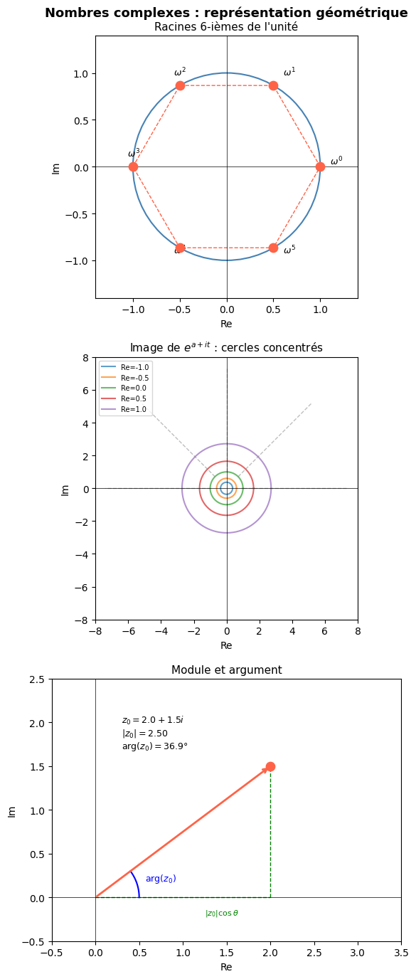
Racines \(n\)-ièmes d’un nombre complexe#

Proposition 321 (Racines \(n\)-ièmes)

Soit \(z_0 \in \mathbb{C}^*\) et \(n \geq 2\). L’équation \(z^n = z_0\) admet exactement \(n\) solutions dans \(\mathbb{C}\),

\[z_k = \sqrt[n]{|z_0|} \, e^{i(\theta_0 + 2k\pi)/n}, \quad k = 0, 1, \ldots, n - 1\]

\(\theta_0 = \arg(z_0)\). Ces \(n\) points forment un polygone régulier inscrit dans le cercle de rayon \(\sqrt[n]{|z_0|}\).

Proof. Avec \(z = re^{i\theta}\), \(r > 0\) : \(r^n = |z_0|\) (unique solution positive) et \(n\theta \equiv \theta_0 \pmod{2\pi}\), soit \(\theta = (\theta_0 + 2k\pi)/n\). Les valeurs distinctes sont \(k = 0, \ldots, n-1\).

Remarque 133

Les racines \(n\)-ièmes de l’unité sont \(\omega^k = e^{2ik\pi/n}\) pour \(k = 0, \ldots, n-1\), où \(\omega = e^{2i\pi/n}\). Elles forment un groupe cyclique \(\mathbb{U}_n\) d’ordre \(n\) pour la multiplication.

Exemple 146

Racines carrées de \(3 + 4i\) : \(|z_0| = 5\), \(\arg(z_0) = \arctan(4/3)\). Méthode algébrique : on cherche \(w = x + iy\) avec \(w^2 = 3 + 4i\).

\[x^2 - y^2 = 3, \quad 2xy = 4, \quad x^2 + y^2 = 5\]

D’où \(x^2 = 4\), \(x = 2\), \(y = 1\). Les racines sont \(\pm(2 + i)\).

Racines carrées sous forme algébrique#

Proposition 322 (Racines carrées en forme algébrique)

Soit \(z_0 = a + ib \in \mathbb{C}^*\). Les racines carrées de \(z_0\) sont \(\pm(x + iy)\)

\[x = \sqrt{\frac{|z_0| + a}{2}}, \qquad y = \frac{b}{2x} \quad \text{si } x \neq 0\]

Si \(b = 0\) et \(a < 0\), alors \(x = 0\) et \(y = \pm\sqrt{-a}\).

Proof. On cherche \(w = x + iy\) tel que \(w^2 = z_0\), soit \(x^2 - y^2 = a\), \(2xy = b\), \(x^2 + y^2 = |z_0|\). En combinant : \(x^2 = (|z_0|+a)/2 \geq 0\), \(y^2 = (|z_0|-a)/2 \geq 0\). Le signe de \(y\) est donné par \(2xy = b\).

Équation du second degré dans \(\mathbb{C}\)#

Proposition 323 (Formule générale)

Soit \(a, b, c \in \mathbb{C}\) avec \(a \neq 0\). L’équation \(az^2 + bz + c = 0\) admet deux solutions (comptées avec multiplicité) :

\[z = \frac{-b \pm \delta}{2a}\]

\(\delta\) est une racine carrée du discriminant \(\Delta = b^2 - 4ac\).

Proof. Par complétion du carré : \(az^2 + bz + c = a\left[(z + b/(2a))^2 - \Delta/(4a^2)\right]\). On conclut en résolvant \((z + b/(2a))^2 = \Delta/(4a^2)\).
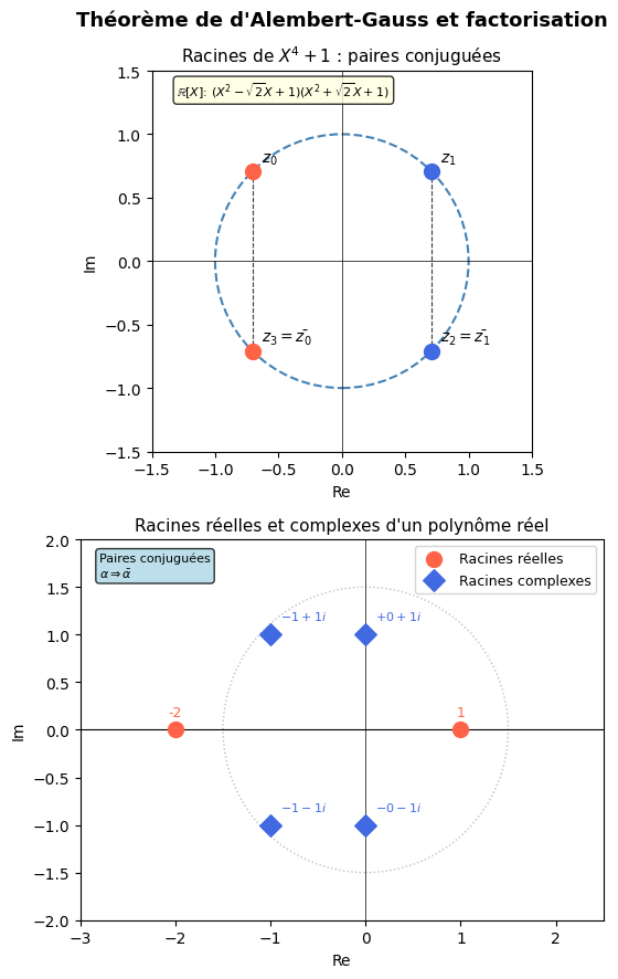
Remarque 134

Si \(a, b, c \in \mathbb{R}\) et \(\Delta < 0\), les deux racines sont complexes conjuguées \(\alpha\) et \(\bar\alpha\). C’est le cas général : si \(P \in \mathbb{R}[X]\) et \(P(\alpha) = 0\), alors \(P(\bar\alpha) = 0\).

Polynômes et clôture algébrique#

Définition 265 (Polynôme à coefficients complexes)

Un polynôme \(P(X) = \sum_{k=0}^n a_k X^k \in \mathbb{C}[X]\) de degré \(n\) (si \(a_n \neq 0\)). La multiplicité d’une racine \(\alpha\) est le plus grand \(m \geq 1\) tel que \((X-\alpha)^m \mid P\).

Proposition 324 (Division euclidienne et critère de racine)

\(\alpha \in \mathbb{C}\) est racine de \(P\) si et seulement si \((X - \alpha)\) divise \(P\). Un polynôme de degré \(n\) a au plus \(n\) racines (avec multiplicités).

Le théorème de d’Alembert-Gauss#

Théorème 69 (Théorème fondamental de l’algèbre)

Tout polynôme \(P \in \mathbb{C}[X]\) de degré \(n \geq 1\) admet au moins une racine dans \(\mathbb{C}\). Donc \(P\) se factorise :

\[P(X) = a_n(X - \alpha_1)^{m_1} \cdots (X - \alpha_r)^{m_r}, \quad m_1 + \cdots + m_r = n\]

On dit que \(\mathbb{C}\) est algébriquement clos.

Proof. Idée analytique. Posons \(P(z) = z^n + \cdots + a_0\). Comme \(|P(z)| \to +\infty\) lorsque \(|z| \to +\infty\), \(|P|\) atteint son minimum en un point \(z_0\). Si \(P(z_0) \neq 0\), en écrivant \(P(z + z_0)/P(z_0) = 1 + a_p z^p + O(z^{p+1})\) et en choisissant \(z = te^{i\theta}\) avec \(a_p e^{ip\theta} < 0\) réel, on obtient \(|P(z_0 + te^{i\theta})| < |P(z_0)|\) pour \(t\) assez petit — contradiction.

Théorème 70 (Factorisation dans \(\mathbb{R}[X]\))

Tout \(P \in \mathbb{R}[X]\) se factorise en produit de facteurs irréductibles de degré 1 ou 2 sur \(\mathbb{R}\) :

\[P(X) = a_n \prod_i (X - r_i)^{m_i} \prod_j (X^2 + p_j X + q_j)^{n_j}\]

où les \(r_i \in \mathbb{R}\), et les facteurs du second degré ont discriminant \(p_j^2 - 4q_j < 0\).

Proof. Les racines non réelles viennent par paires conjuguées \((\alpha, \bar\alpha)\), et \((X - \alpha)(X - \bar\alpha) = X^2 - 2\operatorname{Re}(\alpha)X + |\alpha|^2 \in \mathbb{R}[X]\) est irréductible.

Hide code cell source

import numpy as np
import matplotlib.pyplot as plt
from matplotlib.patches import FancyArrowPatch

fig, axes = plt.subplots(2, 1, figsize=(9, 9))

# --- Racines de X^4 + 1 ---
ax = axes[0]
coeffs = [1, 0, 0, 0, 1]  # X^4 + 1
roots = np.roots(coeffs)

circle = plt.Circle((0,0), 1, fill=False, color='steelblue', lw=1.5, linestyle='--')
ax.add_patch(circle)
colors = ['tomato', 'tomato', 'royalblue', 'royalblue']
labels_r = ['$z_0$', '$z_3=\\bar{z_0}$', '$z_1$', '$z_2=\\bar{z_1}$']

for i, (r, c, lbl) in enumerate(zip(roots, colors, labels_r)):
    ax.scatter([r.real], [r.imag], color=c, s=100, zorder=5)
    ax.annotate(lbl, (r.real, r.imag), xytext=(r.real+0.07, r.imag+0.07), fontsize=10)

# Paires conjuguées
for r in roots:
    ax.plot([r.real, r.real], [r.imag, -r.imag], 'k--', lw=0.8, alpha=0.5)

ax.set_xlim(-1.5, 1.5); ax.set_ylim(-1.5, 1.5)
ax.set_aspect('equal')
ax.axhline(0, color='k', lw=0.5); ax.axvline(0, color='k', lw=0.5)
ax.set_title('Racines de $X^4+1$ : paires conjuguées', fontsize=11)
ax.set_xlabel('Re'); ax.set_ylabel('Im')
ax.text(-1.3, 1.3, '$\\mathbb{R}[X]$: $(X^2-\\sqrt{2}X+1)(X^2+\\sqrt{2}X+1)$', fontsize=8,
        bbox=dict(boxstyle='round', facecolor='lightyellow', alpha=0.8))

# --- Polynôme de degré 5, zéros et factorisation ---
ax = axes[1]
# P(X) = (X-1)(X+2)(X^2+1)(X^2+2X+2)
# Roots: 1, -2, ±i, -1±i
real_roots = np.array([1, -2])
complex_roots = np.array([1j, -1j, -1+1j, -1-1j])

ax.scatter(real_roots, np.zeros_like(real_roots), color='tomato', s=100, zorder=5, label='Racines réelles')
ax.scatter(complex_roots.real, complex_roots.imag, color='royalblue', s=100, zorder=5, marker='D', label='Racines complexes')

for r in real_roots:
    ax.annotate(f'{r}', (r, 0), xytext=(r, 0.15), ha='center', fontsize=9, color='tomato')
for r in complex_roots:
    ax.annotate(f'${r.real:+.0f}{r.imag:+.0f}i$', (r.real, r.imag),
                xytext=(r.real+0.1, r.imag+0.15), fontsize=8, color='royalblue')

circle = plt.Circle((0,0), 1.5, fill=False, color='gray', lw=1, linestyle=':', alpha=0.5)
ax.add_patch(circle)

ax.set_xlim(-3, 2.5); ax.set_ylim(-2, 2)
ax.set_aspect('equal')
ax.axhline(0, color='k', lw=0.8); ax.axvline(0, color='k', lw=0.5)
ax.set_title('Racines réelles et complexes d\'un polynôme réel', fontsize=11)
ax.set_xlabel('Re'); ax.set_ylabel('Im')
ax.legend(fontsize=9)
ax.text(-2.8, 1.6, 'Paires conjuguées\n$\\alpha \\Rightarrow \\bar{\\alpha}$', fontsize=8,
        bbox=dict(boxstyle='round', facecolor='lightblue', alpha=0.8))

plt.suptitle('Théorème de d\'Alembert-Gauss et factorisation', fontsize=13, fontweight='bold')
plt.tight_layout()
plt.show()
_images/fe9f2847c531598078e221506423e25b39779e859a660cbed1f66fb1c7154622.png

Relations coefficients-racines : formules de Viète#

Théorème 71 (Formules de Viète)

Soit \(P(X) = a_n X^n + \cdots + a_0\) de racines \(\alpha_1, \ldots, \alpha_n\) (avec multiplicité). Si \(\sigma_k\) est la \(k\)-ième fonction symétrique élémentaire :

\[\sigma_k(\alpha_1, \ldots, \alpha_n) = \sum_{1 \leq i_1 < \cdots < i_k \leq n} \alpha_{i_1} \cdots \alpha_{i_k} = (-1)^k \frac{a_{n-k}}{a_n}\]

En particulier : \(\sum_i \alpha_i = -a_{n-1}/a_n\) et \(\prod_i \alpha_i = (-1)^n a_0/a_n\).

Proof. En développant \(a_n \prod_{k=1}^n (X - \alpha_k)\), le coefficient de \(X^{n-k}\) est \(a_n \cdot (-1)^k \sigma_k\).

Exemple 147

Pour \(P(X) = X^3 - 6X^2 + 11X - 6\) de racines \(1, 2, 3\) : \(1+2+3 = 6\), \(1 \cdot 2 + 1 \cdot 3 + 2 \cdot 3 = 11\), \(1 \cdot 2 \cdot 3 = 6\). \(\checkmark\)

Application : si \(\alpha + \beta = S\) et \(\alpha\beta = P\), alors \(\alpha\) et \(\beta\) sont racines de \(X^2 - SX + P\).

Logarithme complexe et caractère multi-valué#

Définition 266 (Logarithme complexe)

Pour \(z \in \mathbb{C}^*\), on définit le logarithme complexe (multi-valué) :

\[\log z = \ln|z| + i\arg(z) = \ln|z| + i(\theta_0 + 2k\pi), \quad k \in \mathbb{Z}\]

La détermination principale correspond à \(\arg(z) \in (-\pi, \pi]\) :

\[\text{Log}\, z = \ln|z| + i\operatorname{Arg}(z), \quad \operatorname{Arg}(z) \in (-\pi, \pi]\]

Remarque 135

Contrairement à l’exponentielle réelle, \(e^z\) n’est pas injective sur \(\mathbb{C}\) (période \(2i\pi\)). Son inverse est donc multi-valué. La détermination principale \(\text{Log}\) est discontinue sur la demi-droite réelle négative (coupure de branche). On a \(e^{\text{Log}\, z} = z\) mais \(\text{Log}(e^z) = z\) seulement si \(\operatorname{Im}(z) \in (-\pi, \pi]\).

Exemple 148

\(\text{Log}(i) = \ln 1 + i\pi/2 = i\pi/2\).

\(\text{Log}(-1) = i\pi\) (mais \(\log(-1) = i\pi + 2ik\pi\), \(k \in \mathbb{Z}\)).

Paradoxe apparent : \(1 = e^0 = e^{2i\pi}\), donc \(\log 1 = 2ik\pi\), \(k \in \mathbb{Z}\) (et non uniquement \(0\)).

Définition 267 (Puissances complexes)

Pour \(a \in \mathbb{C}^*\) et \(b \in \mathbb{C}\), on pose \(a^b = e^{b \log a}\), qui est en général multi-valué. La détermination principale est \(a^b = e^{b \,\text{Log}\, a}\).

Exemple 149

\(i^i = e^{i \cdot \text{Log}\, i} = e^{i \cdot i\pi/2} = e^{-\pi/2} \approx 0.2079\ldots\) : un nombre réel !

Plus généralement \(i^i = e^{i(i\pi/2 + 2ik\pi)} = e^{-\pi/2 - 2k\pi}\), \(k \in \mathbb{Z}\).

Exponentielle complexe#

Proposition 325 (Propriétés)

\(\forall z, w \in \mathbb{C}\) : \(e^{z+w} = e^z e^w\), \(|e^z| = e^{\operatorname{Re}(z)}\), \(\overline{e^z} = e^{\bar z}\), \(e^z = 1 \iff z = 2ik\pi\) (\(k \in \mathbb{Z}\)).

Remarque 136

L’exponentielle complexe est périodique de période \(2i\pi\). L’application \(\mathbb{R} \to \mathbb{U} = \{z : |z| = 1\}\), \(\theta \mapsto e^{i\theta}\), est un morphisme de groupes surjectif de noyau \(2\pi\mathbb{Z}\).

Géométrie dans \(\mathbb{C}\)#

Transformations du plan#

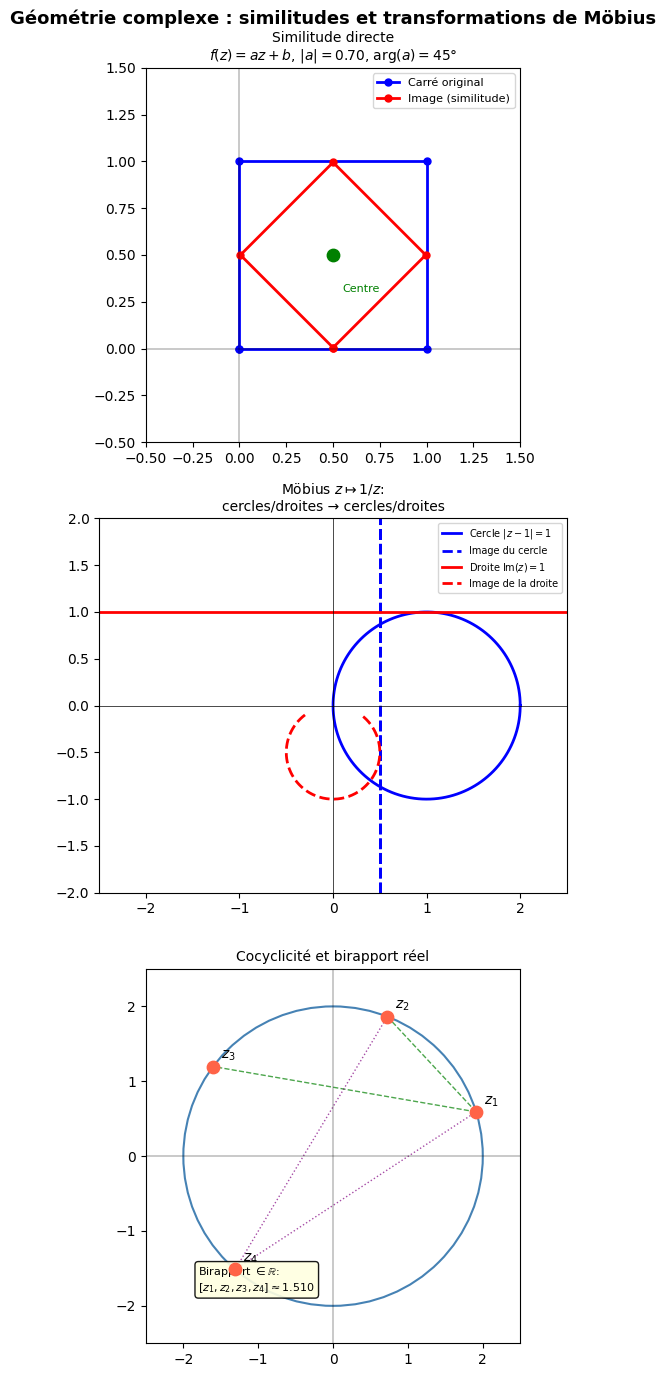
Proposition 326 (Translations, rotations, similitudes)

  • Translation de vecteur \(b\) : \(f(z) = z + b\)

  • Rotation de centre \(\omega\), angle \(\theta\) : \(f(z) = e^{i\theta}(z - \omega) + \omega\)

  • Homothétie de centre \(\omega\), rapport \(r > 0\) : \(f(z) = r(z - \omega) + \omega\)

  • Similitude directe : \(f(z) = az + b\) avec \(a \in \mathbb{C}^*\), \(b \in \mathbb{C}\) (rapport \(|a|\), angle \(\arg(a)\))

  • Similitude indirecte : \(f(z) = a\bar{z} + b\) (renverse l’orientation)

Proof. Pour la rotation : \(|f(z) - f(w)| = |e^{i\theta}(z-w)| = |z-w|\) (isométrie), et \(f\) est directe car \(a = e^{i\theta} \neq 0\). Pour l’angle : \(\arg(f(z)-f(\omega)) = \arg(e^{i\theta}(z-\omega)) = \theta + \arg(z-\omega)\).

Exemple 150

Rotation d’angle \(\pi/2\) autour de \(1+i\) : \(f(z) = e^{i\pi/2}(z - 1 - i) + 1 + i = i(z-1-i) + 1 + i = iz + 2\).

Vérification : \(f(1+i) = i(1+i) + 2 = i - 1 + 2 = 1 + i\) (point fixe). \(\checkmark\)

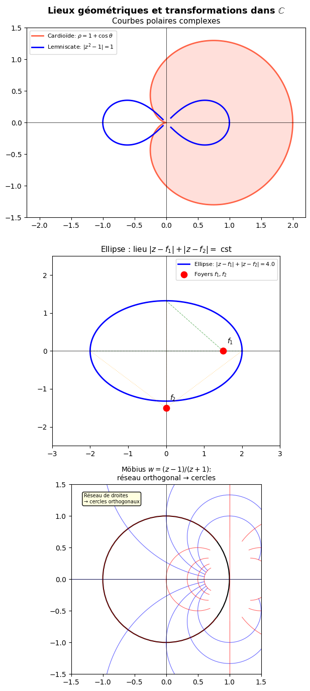
Transformations de Möbius#

Définition 268 (Transformation de Möbius (homographie))

Une transformation de Möbius est une application \(f : \hat{\mathbb{C}} \to \hat{\mathbb{C}}\) (sphère de Riemann \(\hat{\mathbb{C}} = \mathbb{C} \cup \{\infty\}\)) de la forme

\[f(z) = \frac{az + b}{cz + d}, \quad a, b, c, d \in \mathbb{C}, \quad ad - bc \neq 0\]

Proposition 327 (Propriétés des transformations de Möbius)

  • Les transformations de Möbius forment un groupe \(PGL_2(\mathbb{C}) \simeq PSL_2(\mathbb{C})\) pour la composition.

  • Elles sont conformes (conservent les angles orientés).

  • Elles transforment cercles et droites en cercles et droites (dans \(\hat{\mathbb{C}}\), les droites sont des cercles passant par \(\infty\)).

  • Elles sont déterminées par l’image de 3 points quelconques.

Proof. La composition correspond au produit matriciel \(\begin{pmatrix} a & b \\ c & d \end{pmatrix}\). La condition \(ad - bc \neq 0\) assure l’inversibilité. La conformité résulte de la holomorphie (voir ci-dessous). Pour les cercles : une homographie se décompose en translations, homotéties, conjugaisons et l’inversion \(z \mapsto 1/z\), qui transforment chacune les cercles/droites en cercles/droites.

Définition 269 (Birapport)

Le birapport de quatre points distincts \(z_1, z_2, z_3, z_4 \in \hat{\mathbb{C}}\) est

\[[z_1, z_2, z_3, z_4] = \frac{(z_3 - z_1)(z_4 - z_2)}{(z_3 - z_2)(z_4 - z_1)}\]

Proposition 328 (Invariance du birapport)

Les transformations de Möbius conservent le birapport : si \(f\) est une homographie, \([f(z_1), f(z_2), f(z_3), f(z_4)] = [z_1, z_2, z_3, z_4]\).

De plus, quatre points sont cocycliques (ou alignés) si et seulement si leur birapport est réel.

Proof. Pour la cocyclicité : le birapport est réel \(\iff\) \(\arg\frac{z_3-z_1}{z_3-z_2} = \arg\frac{z_4-z_1}{z_4-z_2} \pmod\pi\), c’est-à-dire les angles inscrits en \(z_3\) et \(z_4\) subtendant \([z_1 z_2]\) sont égaux — critère du théorème de l’angle inscrit.

Conditions géométriques#

Proposition 329 (Alignement et angles)

  • Trois points \(a, b, c\) distincts sont alignés \(\iff\) \((c-a)/(b-a) \in \mathbb{R}\)

  • L’angle orienté \((\vec{AB}, \vec{AC}) = \arg\dfrac{c-a}{b-a} \pmod{2\pi}\)

  • Le milieu de \([AB]\) a affixe \((a+b)/2\)

  • Le barycentre de \((A_k, \lambda_k)\) a affixe \(\dfrac{\sum \lambda_k a_k}{\sum \lambda_k}\)

Hide code cell source

import numpy as np
import matplotlib.pyplot as plt
from matplotlib.patches import Arc

fig, axes = plt.subplots(3, 1, figsize=(9, 14))

# --- Similitude : rotation + homothétie ---
ax = axes[0]
# Carré de base
sq = np.array([0, 1, 1+1j, 1j, 0])
center = 0.5 + 0.5j
a = 0.7 * np.exp(1j*np.pi/4)  # similitude
b = (1 - a) * center

sq2 = a * sq + b  # image

ax.plot(sq.real, sq.imag, 'b-o', lw=2, label='Carré original', markersize=5)
ax.plot(sq2.real, sq2.imag, 'r-o', lw=2, label='Image (similitude)', markersize=5)
ax.scatter([center.real], [center.imag], color='green', s=80, zorder=5)
ax.annotate('Centre', (center.real, center.imag), xytext=(0.55, 0.3), fontsize=8, color='green')
ax.set_xlim(-0.5, 1.5); ax.set_ylim(-0.5, 1.5)
ax.set_aspect('equal')
ax.axhline(0, color='k', lw=0.3); ax.axvline(0, color='k', lw=0.3)
ax.set_title(f'Similitude directe\n$f(z)=az+b$, $|a|={abs(a):.2f}$, $\\arg(a)=45°$', fontsize=10)
ax.legend(fontsize=8)

# --- Transformation de Möbius : z -> 1/z ---
ax = axes[1]
theta = np.linspace(0, 2*np.pi, 300)

# Cercle |z-1| = 1 -> image par 1/z
z_circ = 1 + np.exp(1j*theta)
w_circ = 1/z_circ  # image

# Droite Im(z) = 1 -> image par 1/z
x = np.linspace(-3, 3, 300)
z_line = x + 1j
w_line = 1/z_line

ax.plot(z_circ.real, z_circ.imag, 'b-', lw=2, label='Cercle $|z-1|=1$')
ax.plot(w_circ.real, w_circ.imag, 'b--', lw=2, label='Image du cercle')
ax.plot(z_line.real, z_line.imag, 'r-', lw=2, label='Droite $\\mathrm{Im}(z)=1$')
ax.plot(w_line.real, w_line.imag, 'r--', lw=2, label='Image de la droite')

ax.set_xlim(-2.5, 2.5); ax.set_ylim(-2, 2)
ax.set_aspect('equal')
ax.axhline(0, color='k', lw=0.5); ax.axvline(0, color='k', lw=0.5)
ax.set_title('Möbius $z\\mapsto 1/z$:\ncercles/droites → cercles/droites', fontsize=10)
ax.legend(fontsize=7)

# --- Cocyclicité et birapport ---
ax = axes[2]
# Quatre points sur un cercle
theta4 = [0.3, 1.2, 2.5, 4.0]
z1, z2, z3, z4 = [2*np.exp(1j*t) for t in theta4]
pts = [z1, z2, z3, z4]
lbls = ['$z_1$', '$z_2$', '$z_3$', '$z_4$']

circle = plt.Circle((0,0), 2, fill=False, color='steelblue', lw=1.5)
ax.add_patch(circle)

for z, lbl in zip(pts, lbls):
    ax.scatter([z.real], [z.imag], s=80, zorder=5, color='tomato')
    ax.annotate(lbl, (z.real, z.imag), xytext=(z.real+0.1, z.imag+0.1), fontsize=10)

# Draw lines between pairs
ax.plot([z1.real, z3.real], [z1.imag, z3.imag], 'g--', lw=1, alpha=0.7)
ax.plot([z1.real, z2.real], [z1.imag, z2.imag], 'g--', lw=1, alpha=0.7)
ax.plot([z4.real, z2.real], [z4.imag, z2.imag], 'purple', lw=1, linestyle=':', alpha=0.7)
ax.plot([z4.real, z1.real], [z4.imag, z1.imag], 'purple', lw=1, linestyle=':', alpha=0.7)

br = (z3-z1)*(z4-z2)/((z3-z2)*(z4-z1))
ax.text(-1.8, -1.8, f'Birapport $\\in \\mathbb{{R}}$:\n$[z_1,z_2,z_3,z_4]\\approx{br.real:.3f}$', fontsize=8,
        bbox=dict(boxstyle='round', facecolor='lightyellow', alpha=0.9))

ax.set_xlim(-2.5, 2.5); ax.set_ylim(-2.5, 2.5)
ax.set_aspect('equal')
ax.axhline(0, color='k', lw=0.3); ax.axvline(0, color='k', lw=0.3)
ax.set_title('Cocyclicité et birapport réel', fontsize=10)

plt.suptitle('Géométrie complexe : similitudes et transformations de Möbius', fontsize=13, fontweight='bold')
plt.tight_layout()
plt.show()
_images/777d013537fdad00e58a93ebad865983365ea32975fd181d0e1dd57b64b2cb71.png

Lieux géométriques#

Exemple 151

  • Cercle : \(\{z : |z - z_0| = R\}\)

  • Médiatrice de \([AB]\) : \(\{z : |z - a| = |z - b|\}\), équation réelle \(\operatorname{Re}((b-a)\bar z) = (|b|^2 - |a|^2)/2\)

  • Droite : \(\{z : \operatorname{Re}(\alpha\bar z) = c\}\) avec \(\alpha \in \mathbb{C}^*\), \(c \in \mathbb{R}\)

  • Ellipse/hyperbole : \(\{z : |z-a| + |z-b| = 2r\}\) ou \(\{z : |z-a| - |z-b| = \text{cst}\}\)

  • Cardioïde : \(\{z = \rho e^{i\theta} : \rho = 1 + \cos\theta\}\)

Hide code cell source

import numpy as np
import matplotlib.pyplot as plt

fig, axes = plt.subplots(3, 1, figsize=(9, 14))

# --- Lieux géométriques classiques ---
theta = np.linspace(0, 2*np.pi, 500)

# Cardioïde
ax = axes[0]
rho = 1 + np.cos(theta)
x = rho * np.cos(theta)
y = rho * np.sin(theta)
ax.fill(x, y, alpha=0.2, color='tomato')
ax.plot(x, y, 'tomato', lw=2, label='Cardioïde: $\\rho=1+\\cos\\theta$')

# Lemniscate de Bernoulli : |z-1||z+1| = 1
theta2 = np.linspace(0, 2*np.pi, 1000)
r2_sq = np.cos(2*theta2)
mask = r2_sq >= 0
rho2 = np.where(mask, np.sqrt(np.maximum(r2_sq, 0)), np.nan)
x2 = rho2 * np.cos(theta2)
y2 = rho2 * np.sin(theta2)
ax.plot(x2, y2, 'b-', lw=2, label='Lemniscate: $|z^2-1|=1$')

ax.set_xlim(-2.2, 2.2); ax.set_ylim(-1.5, 1.5)
ax.set_aspect('equal')
ax.axhline(0, color='k', lw=0.5); ax.axvline(0, color='k', lw=0.5)
ax.set_title('Courbes polaires complexes', fontsize=11)
ax.legend(fontsize=8)

# --- Ellipse comme lieu complexe ---
ax = axes[1]
a_f, b_f = 1.5, -1.5j  # foyers
r_sum = 4.0  # somme des distances

t = np.linspace(0, 2*np.pi, 500)
a_ell = r_sum/2
c_ell = abs(a_f)  # demi-distance focale
b_ell = np.sqrt(a_ell**2 - c_ell**2)

x_ell = a_ell * np.cos(t)
y_ell = b_ell * np.sin(t)

ax.plot(x_ell, y_ell, 'b-', lw=2, label=f'Ellipse: $|z-f_1|+|z-f_2|={r_sum}$')
ax.scatter([a_f.real, b_f.real], [a_f.imag, b_f.imag],
           color='red', s=80, zorder=5, label='Foyers $f_1, f_2$')
ax.annotate('$f_1$', (a_f.real, a_f.imag), xytext=(a_f.real+0.1, a_f.imag+0.2), fontsize=10)
ax.annotate('$f_2$', (b_f.real, b_f.imag), xytext=(b_f.real+0.1, b_f.imag+0.2), fontsize=10)

# Quelques rayons
for z in [a_ell + 0j, 0 + b_ell*1j, -a_ell + 0j]:
    ax.plot([z.real, a_f.real], [z.imag, a_f.imag], 'g--', lw=0.8, alpha=0.5)
    ax.plot([z.real, b_f.real], [z.imag, b_f.imag], 'orange', lw=0.8, linestyle=':', alpha=0.5)

ax.set_xlim(-3, 3); ax.set_ylim(-2.5, 2.5)
ax.set_aspect('equal')
ax.axhline(0, color='k', lw=0.5); ax.axvline(0, color='k', lw=0.5)
ax.set_title('Ellipse : lieu $|z-f_1|+|z-f_2|=$ cst', fontsize=11)
ax.legend(fontsize=8)

# --- Transformée de Möbius d'un réseau ---
ax = axes[2]
# Image de lignes horizontales et verticales par z -> (z-1)/(z+1)
for im_val in np.linspace(-2, 2, 9):
    x_vals = np.linspace(-4, 4, 300)
    z = x_vals + 1j*im_val
    w = (z - 1)/(z + 1)
    ax.plot(w.real, w.imag, 'b-', lw=0.8, alpha=0.6)

for re_val in np.linspace(-4, 4, 9):
    y_vals = np.linspace(-3, 3, 300)
    z = re_val + 1j*y_vals
    w = (z - 1)/(z + 1)
    ax.plot(w.real, w.imag, 'r-', lw=0.8, alpha=0.6)

circle_u = plt.Circle((0,0), 1, fill=False, color='k', lw=1.5)
ax.add_patch(circle_u)

ax.set_xlim(-1.5, 1.5); ax.set_ylim(-1.5, 1.5)
ax.set_aspect('equal')
ax.axhline(0, color='k', lw=0.5); ax.axvline(0, color='k', lw=0.5)
ax.set_title('Möbius $w=(z-1)/(z+1)$:\nréseau orthogonal → cercles', fontsize=10)
ax.text(-1.3, 1.2, 'Réseau de droites\n→ cercles orthogonaux', fontsize=7,
        bbox=dict(boxstyle='round', facecolor='lightyellow'))

plt.suptitle('Lieux géométriques et transformations dans $\\mathbb{C}$', fontsize=13, fontweight='bold')
plt.tight_layout()
plt.show()
_images/718ccb3d505497d67483547c3137746de4e00910a0bf70c7b364de85b7dacedd.png

Topologie de \(\mathbb{C}\) et aperçu analytique#

Définition 270 (Structure topologique de \(\mathbb{C}\))

On identifie \(\mathbb{C} \simeq \mathbb{R}^2\) via \(z = x + iy \leftrightarrow (x, y)\), muni de la distance \(d(z, w) = |z - w|\).

  • Disque ouvert : \(D(z_0, r) = \{z : |z - z_0| < r\}\)

  • Ensemble ouvert : \(U\) tel que tout point de \(U\) est centre d’un disque inclus dans \(U\)

  • Ensemble connexe : non décomposable en deux ouverts disjoints non vides

Proposition 330 (Convergence dans \(\mathbb{C}\))

\((z_n) \to \ell = a + ib\) si et seulement si \(\operatorname{Re}(z_n) \to a\) et \(\operatorname{Im}(z_n) \to b\). La convergence absolue d’une série complexe implique sa convergence.

Définition 271 (Fonction holomorphe (aperçu))

Une fonction \(f : U \subset \mathbb{C} \to \mathbb{C}\) est holomorphe en \(z_0 \in U\) si la limite

\[f'(z_0) = \lim_{h \to 0} \frac{f(z_0 + h) - f(z_0)}{h}\]

existe dans \(\mathbb{C}\). L’holomorphie est une condition bien plus forte que la différentiabilité réelle — elle implique l’analyticité (développabilité en série entière).

Remarque 137

Les polynômes, \(e^z\), \(\sin z\), \(\cos z\) sont holomorphes sur \(\mathbb{C}\) entier (fonctions entières). La fonction \(z \mapsto \bar z\) n’est pas holomorphe. Les transformations de Möbius sont holomorphes sur \(\hat{\mathbb{C}} \setminus \{-d/c\}\).

Les équations de Cauchy-Riemann caractérisent l’holomorphie : si \(f = u + iv\), alors \(f\) holomorphe \(\iff\) \(\partial_x u = \partial_y v\) et \(\partial_x v = -\partial_y u\).

Résumé#

Concept

Résultat clé

Racines \(n\)-ièmes

\(n\) racines : polygone régulier

d’Alembert-Gauss

\(\mathbb{C}\) algébriquement clos, factorisation complète

Polynômes réels

Racines conjuguées, facteurs deg 1 et 2

Formules de Viète

\(\sigma_k = (-1)^k a_{n-k}/a_n\)

Logarithme

Multi-valué, coupure de branche, \(i^i \in \mathbb{R}\)

Similitudes

\(f(z) = az + b\) ; rapport $

Möbius

Conserve angles et cercles/droites, birapport

Cocyclicité

Birapport réel

Holomorphie

Cauchy-Riemann, analyticité