Variables aléatoires continues

Dieu ne joue pas aux dés… mais il en lance quand même à chaque instant.

Albert Einstein (paraphrase)

Introduction

Le chapitre précédent étudiait les variables aléatoires prenant un nombre fini ou dénombrable de valeurs. De nombreux phénomènes — durée de vie, mesure physique, position d’une particule — prennent des valeurs dans un continuum. Ce chapitre développe la théorie des variables aléatoires continues, caractérisées par une densité de probabilité.

Show code cell source

Hide code cell source

import numpy as np
import matplotlib.pyplot as plt
import seaborn as sns
from scipy import stats, integrate

sns.set_theme(style="whitegrid", palette="muted", font_scale=1.1)

fig, axes = plt.subplots(3, 1, figsize=(9, 14))

# 1. Lois continues classiques : densités
x = np.linspace(-4, 6, 500)
ax = axes[0]
# Uniforme [0,2]
xu = np.linspace(-0.5, 2.5, 500)
ax.plot(xu, stats.uniform.pdf(xu, 0, 2), 'steelblue', lw=2, label='$\\mathcal{U}([0,2])$')
# Exponentielle lambda=1
xe = np.linspace(0, 5, 400)
ax.plot(xe, stats.expon.pdf(xe), 'tomato', lw=2, label='$\\mathcal{E}(1)$')
# Normale(1, 0.5^2)
ax.plot(x, stats.norm.pdf(x, 1, 0.5), 'gold', lw=2, label='$\\mathcal{N}(1, 0.25)$')
# Gamma(2, 1)
xg = np.linspace(0, 6, 400)
ax.plot(xg, stats.gamma.pdf(xg, 2, scale=1), 'green', lw=2, label='$\\Gamma(2,1)$')
ax.set_xlabel('$x$'); ax.set_ylabel('$f(x)$')
ax.set_title('Densités des lois continues classiques')
ax.legend(fontsize=9); ax.set_xlim(-0.5, 5); ax.set_ylim(0, 2.2)

# 2. Fonctions de répartition correspondantes
ax = axes[1]
ax.plot(xu, stats.uniform.cdf(xu, 0, 2), 'steelblue', lw=2, label='$\\mathcal{U}([0,2])$')
ax.plot(xe, stats.expon.cdf(xe), 'tomato', lw=2, label='$\\mathcal{E}(1)$')
ax.plot(x, stats.norm.cdf(x, 1, 0.5), 'gold', lw=2, label='$\\mathcal{N}(1, 0.25)$')
ax.plot(xg, stats.gamma.cdf(xg, 2, scale=1), 'green', lw=2, label='$\\Gamma(2,1)$')
ax.axhline(0.5, color='gray', lw=0.8, linestyle='--', alpha=0.6)
ax.set_xlabel('$x$'); ax.set_ylabel('$F(x)$')
ax.set_title('Fonctions de répartition\n$F(x) = \\mathbb{P}(X \\leq x)$')
ax.legend(fontsize=9); ax.set_xlim(-0.5, 5)

# 3. Intégrale de Gauss I^2 = pi : visualisation 3D réduite à 2D
ax = axes[2]
r = np.linspace(0, 3, 200)
# Intégrale en polaires : I^2 = int_0^infty 2*pi*r*e^{-r^2} dr
integrand = 2 * np.pi * r * np.exp(-r**2)
cumul = np.array([integrate.quad(lambda t: 2*np.pi*t*np.exp(-t**2), 0, rv)[0] for rv in r])
ax.plot(r, integrand, 'steelblue', lw=2, label='$2\\pi r e^{-r^2}$ (intégrand polaire)')
ax.fill_between(r, 0, integrand, alpha=0.2, color='steelblue')
ax.plot(r, cumul, 'tomato', lw=2, label='Intégrale cumulée $\\to \\pi$')
ax.axhline(np.pi, color='tomato', lw=1, linestyle='--', alpha=0.6)
ax.text(2.5, np.pi + 0.05, '$I^2 = \\pi$', color='tomato', fontsize=11)
# Annoter le calcul
ax.text(0.5, 1.8, '$I = \\int_{-\\infty}^{+\\infty} e^{-x^2}dx$\n$I^2 = \\iint e^{-(x^2+y^2)}dxdy$\n$= 2\\pi\\int_0^\\infty re^{-r^2}dr = \\pi$\n$I = \\sqrt{\\pi}$',
        fontsize=9, bbox=dict(boxstyle='round', fc='white', alpha=0.8))
ax.set_xlabel('$r$'); ax.set_ylabel('Valeur')
ax.set_title("Intégrale de Gauss par coordonnées polaires\n$\\int e^{-x^2}dx = \\sqrt{\\pi}$")
ax.legend(fontsize=9)

plt.tight_layout()
plt.show()

Variables aléatoires à densité

Définition 283 (Fonction de répartition)

La fonction de répartition d’une variable aléatoire réelle \(X\) est

\[F_X(x) = \mathbb{P}(X \leq x), \quad x \in \mathbb{R}\]

Proposition 338 (Propriétés de la fonction de répartition)

1. \(F\) est croissante

2. \(F\) est continue à droite : \(F(x^+) = F(x)\)

3. \(\lim_{x \to -\infty} F(x) = 0\) et \(\lim_{x \to +\infty} F(x) = 1\)

4. \(\mathbb{P}(a < X \leq b) = F(b) - F(a)\)

5. Les sauts de \(F\) en \(x\) valent \(\mathbb{P}(X = x)\)

Définition 284 (Variable aléatoire à densité)

\(X\) est une variable aléatoire à densité s’il existe \(f_X : \mathbb{R} \to \mathbb{R}_+\) intégrable telle que

\[F_X(x) = \int_{-\infty}^x f_X(t) \, dt \quad \forall x \in \mathbb{R}\]

La fonction \(f_X\) est la densité de \(X\).

Proposition 339 (Propriétés de la densité)

• \(f_X \geq 0\) et \(\int_{-\infty}^{+\infty} f_X(t) \, dt = 1\)

• \(F_X\) est continue (donc \(\mathbb{P}(X = x) = 0\) pour tout \(x\))

• \(F_X\) est dérivable p.p. et \(F_X' = f_X\)

• \(\mathbb{P}(a \leq X \leq b) = \mathbb{P}(a < X < b) = \int_a^b f_X(t) \, dt\)

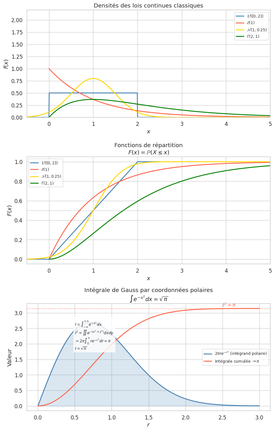
Lois continues classiques

Définition 285 (Loi uniforme \(\mathcal{U}([a,b])\))

\[f(x) = \frac{1}{b-a}\mathbf{1}_{[a,b]}(x)\]

\(\mathbb{E}[X] = (a+b)/2\), \(\text{Var}(X) = (b-a)^2/12\).

Définition 286 (Loi exponentielle \(\mathcal{E}(\lambda)\))

\[f(x) = \lambda e^{-\lambda x}\mathbf{1}_{x \geq 0}, \quad \lambda > 0, \quad F(x) = (1 - e^{-\lambda x})\mathbf{1}_{x \geq 0}\]

\(\mathbb{E}[X] = 1/\lambda\), \(\text{Var}(X) = 1/\lambda^2\).

Modélise les durées de vie, les temps d’attente (processus de Poisson).

Proposition 340 (Absence de mémoire de l’exponentielle)

La loi exponentielle est l’unique loi continue vérifiant :

\[\mathbb{P}(X > s + t \mid X > s) = \mathbb{P}(X > t)\]

Proof. \(\mathbb{P}(X > t) = e^{-\lambda t}\). Donc \(\mathbb{P}(X > s+t \mid X > s) = e^{-\lambda(s+t)}/e^{-\lambda s} = e^{-\lambda t} = \mathbb{P}(X > t)\).

Unicité : Si \(g(t) = \mathbb{P}(X > t)\) est continue et vérifie \(g(s+t) = g(s)g(t)\) avec \(g(0) = 1\), \(g\) décroissante, alors \(g(t) = e^{-\lambda t}\) pour un \(\lambda \geq 0\) (les seules solutions continues de l’équation de Cauchy multiplicative).

Définition 287 (Loi normale \(\mathcal{N}(\mu, \sigma^2)\))

\[f(x) = \frac{1}{\sigma\sqrt{2\pi}} \exp\!\left(-\frac{(x-\mu)^2}{2\sigma^2}\right)\]

\(\mu \in \mathbb{R}\) est la moyenne, \(\sigma > 0\) l’écart-type. La loi normale centrée réduite est \(\mathcal{N}(0,1)\) : \(f(x) = \frac{1}{\sqrt{2\pi}}e^{-x^2/2}\).

Proposition 341 (Intégrabilité)

\(\int_{-\infty}^{+\infty} \frac{1}{\sqrt{2\pi}} e^{-x^2/2} dx = 1\).

Proof. Par le changement de variables \(x = t/\sqrt{2}\) dans l’intégrale de Gauss : \(\int_{-\infty}^{+\infty} e^{-x^2} dx = \sqrt{\pi}\) (calculée au chapitre 31 par coordonnées polaires). Donc \(\int e^{-t^2/2} dt/\sqrt{2} = \sqrt{\pi}\), soit \(\int e^{-t^2/2} dt = \sqrt{2\pi}\).

Définition 288 (Loi gamma \(\Gamma(\alpha, \lambda)\))

\[f(x) = \frac{\lambda^\alpha}{\Gamma(\alpha)} x^{\alpha-1} e^{-\lambda x} \mathbf{1}_{x > 0}, \quad \alpha, \lambda > 0\]

où \(\Gamma(\alpha) = \int_0^{+\infty} t^{\alpha-1} e^{-t} dt\) est la fonction gamma (\(\Gamma(n) = (n-1)!\)).

• \(\Gamma(1, \lambda) = \mathcal{E}(\lambda)\)

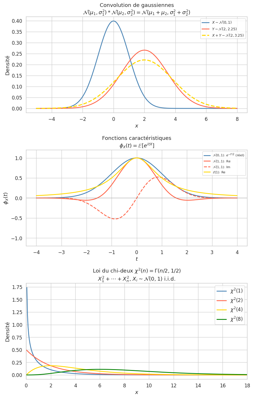
• \(\Gamma(n/2, 1/2) = \chi^2(n)\) (loi du chi-deux à \(n\) degrés de liberté)

• Stable par somme : si \(X \sim \Gamma(\alpha, \lambda)\), \(Y \sim \Gamma(\beta, \lambda)\) indépendantes, alors \(X+Y \sim \Gamma(\alpha+\beta, \lambda)\)

Proposition 342 (Espérance et variance des lois classiques)

Loi	\(\mathbb{E}[X]\)	\(\text{Var}(X)\)
\(\mathcal{U}([a,b])\)	\((a+b)/2\)	\((b-a)^2/12\)
\(\mathcal{E}(\lambda)\)	\(1/\lambda\)	\(1/\lambda^2\)
\(\mathcal{N}(\mu, \sigma^2)\)	\(\mu\)	\(\sigma^2\)
\(\Gamma(\alpha, \lambda)\)	\(\alpha/\lambda\)	\(\alpha/\lambda^2\)

Proof. Exponentielle : \(\mathbb{E}[X] = \int_0^\infty x\lambda e^{-\lambda x}dx\). Par IPP : \(= [-xe^{-\lambda x}]_0^\infty + \int_0^\infty e^{-\lambda x}dx = 1/\lambda\). \(\mathbb{E}[X^2] = 2/\lambda^2\) (double IPP). \(\text{Var}(X) = 2/\lambda^2 - 1/\lambda^2 = 1/\lambda^2\).

Normale centrée réduite : \(\mathbb{E}[X] = 0\) (intégrande impaire). \(\mathbb{E}[X^2] = \frac{1}{\sqrt{2\pi}}\int x^2 e^{-x^2/2}dx\). Par IPP (\(u = x\), \(dv = xe^{-x^2/2}dx\)) : \(\int x^2 e^{-x^2/2}dx = [-xe^{-x^2/2}]_{-\infty}^{+\infty} + \int e^{-x^2/2}dx = \sqrt{2\pi}\). Donc \(\mathbb{E}[X^2] = 1\).

Densité d’une fonction de variable aléatoire

Théorème 77 (Changement de variable)

Si \(X\) a pour densité \(f_X\) et \(g : \mathbb{R} \to \mathbb{R}\) est un difféomorphisme de classe \(\mathcal{C}^1\), alors \(Y = g(X)\) a pour densité

\[f_Y(y) = f_X(g^{-1}(y)) \cdot |(g^{-1})'(y)|\]

Proof. Pour \(g\) strictement croissante : \(F_Y(y) = \mathbb{P}(g(X) \leq y) = \mathbb{P}(X \leq g^{-1}(y)) = F_X(g^{-1}(y))\). En dérivant : \(f_Y(y) = f_X(g^{-1}(y)) \cdot (g^{-1})'(y)\). Pour \(g\) strictement décroissante, on obtient un signe \(-\), d’où la valeur absolue.

Exemple 154

Si \(X \sim \mathcal{N}(0,1)\), alors \(Y = \mu + \sigma X \sim \mathcal{N}(\mu, \sigma^2)\). \(g^{-1}(y) = (y-\mu)/\sigma\), \((g^{-1})'(y) = 1/\sigma\). \(f_Y(y) = \frac{1}{\sqrt{2\pi}}e^{-(y-\mu)^2/(2\sigma^2)} \cdot \frac{1}{\sigma}\). ✓

Vecteurs aléatoires continus

Définition 289 (Densité conjointe)

\((X, Y)\) est un vecteur aléatoire continu s’il admet une densité conjointe \(f_{X,Y} : \mathbb{R}^2 \to \mathbb{R}_+\) telle que

\[\mathbb{P}((X,Y) \in A) = \iint_A f_{X,Y}(x,y) \, dx \, dy\]

Définition 290 (Densités marginales et indépendance)

\[f_X(x) = \int_{-\infty}^{+\infty} f_{X,Y}(x,y) \, dy, \qquad f_Y(y) = \int_{-\infty}^{+\infty} f_{X,Y}(x,y) \, dx\]

\(X\) et \(Y\) sont indépendantes \(\iff\) \(f_{X,Y}(x,y) = f_X(x) \cdot f_Y(y)\) pour tout \((x,y)\).

Somme de variables indépendantes : convolution

Théorème 78 (Densité d’une somme)

Si \(X, Y\) sont indépendantes de densités \(f_X, f_Y\), alors \(Z = X + Y\) a pour densité

\[f_Z(z) = (f_X * f_Y)(z) = \int_{-\infty}^{+\infty} f_X(t) f_Y(z-t) \, dt\]

Proof. \(F_Z(z) = \mathbb{P}(X+Y \leq z) = \iint_{x+y \leq z} f_X(x)f_Y(y) \, dx \, dy = \int f_X(x)\left(\int_{-\infty}^{z-x} f_Y(y)dy\right) dx\). En dérivant par rapport à \(z\) (dérivation sous le signe intégral) : \(f_Z(z) = \int f_X(x) f_Y(z-x) dx\).

Exemple 155

• \(X \sim \mathcal{N}(\mu_1, \sigma_1^2)\), \(Y \sim \mathcal{N}(\mu_2, \sigma_2^2)\) indépendantes \(\implies X+Y \sim \mathcal{N}(\mu_1+\mu_2, \sigma_1^2+\sigma_2^2)\)

  Preuve : Par les fonctions caractéristiques : \(\phi_{X+Y}(t) = e^{i\mu_1 t - \sigma_1^2 t^2/2} \cdot e^{i\mu_2 t - \sigma_2^2 t^2/2} = e^{i(\mu_1+\mu_2)t - (\sigma_1^2+\sigma_2^2)t^2/2}\).

• \(X \sim \mathcal{E}(\lambda)\), \(Y \sim \mathcal{E}(\lambda)\) indépendantes \(\implies X+Y \sim \Gamma(2,\lambda)\)

Fonction caractéristique

Définition 291 (Fonction caractéristique)

La fonction caractéristique de \(X\) est

\[\phi_X(t) = \mathbb{E}[e^{itX}] = \int_{-\infty}^{+\infty} e^{itx} f_X(x) \, dx, \quad t \in \mathbb{R}\]

C’est la transformée de Fourier de la densité.

Proposition 343 (Propriétés)

• \(\phi_X(0) = 1\) et \(|\phi_X(t)| \leq 1\)

• \(\phi_X\) détermine uniquement la loi de \(X\) (injectivité de la transformée de Fourier)

• \(X, Y\) indépendantes \(\implies \phi_{X+Y}(t) = \phi_X(t) \cdot \phi_Y(t)\)

• \(\mathbb{E}[X^k] = \frac{\phi_X^{(k)}(0)}{i^k}\) (si le moment d’ordre \(k\) existe)

• Continuité : \(X_n \xrightarrow{\mathcal{L}} X \iff \phi_{X_n}(t) \to \phi_X(t)\) pour tout \(t\) (théorème de Lévy)

Exemple 156

• \(\mathcal{N}(0,1)\) : \(\phi(t) = e^{-t^2/2}\) (la gaussienne est sa propre transformée de Fourier à normalisation près)

• \(\mathcal{N}(\mu,\sigma^2)\) : \(\phi(t) = e^{i\mu t - \sigma^2 t^2/2}\)

• \(\mathcal{E}(\lambda)\) : \(\phi(t) = \frac{\lambda}{\lambda - it}\)

• \(\mathcal{P}(\lambda)\) : \(\phi(t) = e^{\lambda(e^{it}-1)}\)

Proof. \(\mathcal{N}(0,1)\) : \(\phi(t) = \frac{1}{\sqrt{2\pi}}\int e^{itx}e^{-x^2/2}dx = \frac{1}{\sqrt{2\pi}}\int e^{-(x-it)^2/2}e^{-t^2/2}dx = e^{-t^2/2}\) (complétion du carré et intégrale de Gauss dans \(\mathbb{C}\)).

Show code cell source

Hide code cell source

fig, axes = plt.subplots(3, 1, figsize=(9, 14))

# 1. Convolution : somme de gaussiennes
ax = axes[0]
x = np.linspace(-5, 8, 500)
f1 = stats.norm.pdf(x, 0, 1)
f2 = stats.norm.pdf(x, 2, 1.5)
f_sum = stats.norm.pdf(x, 2, np.sqrt(1 + 1.5**2))
ax.plot(x, f1, 'steelblue', lw=2, label='$X \\sim \\mathcal{N}(0,1)$')
ax.plot(x, f2, 'tomato', lw=2, label='$Y \\sim \\mathcal{N}(2,2.25)$')
ax.plot(x, f_sum, 'gold', lw=2.5, linestyle='--', label='$X+Y \\sim \\mathcal{N}(2, 3.25)$')
ax.set_xlabel('$x$'); ax.set_ylabel('Densité')
ax.set_title('Convolution de gaussiennes\n$\\mathcal{N}(\\mu_1,\\sigma_1^2)*\\mathcal{N}(\\mu_2,\\sigma_2^2) = \\mathcal{N}(\\mu_1+\\mu_2, \\sigma_1^2+\\sigma_2^2)$')
ax.legend(fontsize=9)

# 2. Fonctions caractéristiques
ax = axes[1]
t = np.linspace(-4, 4, 400)
# N(0,1) : phi = exp(-t^2/2)
phi_n01_re = np.exp(-t**2/2)
phi_n01_im = np.zeros_like(t)
# N(1, 1) : phi = exp(it - t^2/2)
phi_n11_re = np.exp(-t**2/2) * np.cos(t)
phi_n11_im = np.exp(-t**2/2) * np.sin(t)
# Exp(1) : phi = 1/(1-it) => re = 1/(1+t^2), im = t/(1+t^2)
phi_e_re = 1/(1+t**2)
phi_e_im = t/(1+t**2)

ax.plot(t, phi_n01_re, 'steelblue', lw=2, label='$\\mathcal{N}(0,1)$: $e^{-t^2/2}$ (réel)')
ax.plot(t, phi_n11_re, 'tomato', lw=2, label='$\\mathcal{N}(1,1)$: Re')
ax.plot(t, phi_n11_im, 'tomato', lw=2, linestyle='--', label='$\\mathcal{N}(1,1)$: Im')
ax.plot(t, phi_e_re, 'gold', lw=2, label='$\\mathcal{E}(1)$: Re')
ax.axhline(0, color='gray', lw=0.5)
ax.set_xlabel('$t$'); ax.set_ylabel('$\\phi_X(t)$')
ax.set_title('Fonctions caractéristiques\n$\\phi_X(t)=\\mathbb{E}[e^{itX}]$')
ax.legend(fontsize=8); ax.set_ylim(-1.2, 1.2)

# 3. Loi chi-deux : somme de normales au carre
ax = axes[2]
x_chi = np.linspace(0, 20, 400)
for dof, color in [(1,'steelblue'),(2,'tomato'),(4,'gold'),(8,'green')]:
    ax.plot(x_chi, stats.chi2.pdf(x_chi, dof), lw=2, color=color, label=f'$\\chi^2({dof})$')
ax.set_xlabel('$x$'); ax.set_ylabel('Densité')
ax.set_title('Loi du chi-deux $\\chi^2(n) = \\Gamma(n/2, 1/2)$\n$X_1^2+\\cdots+X_n^2$, $X_i \\sim \\mathcal{N}(0,1)$ i.i.d.')
ax.legend(); ax.set_xlim(0, 18)

plt.tight_layout()
plt.show()

Résumé

Concept	Formule / Propriété
Densité	\(f \geq 0\), \(\int f = 1\), \(\mathbb{P}(a \leq X \leq b) = \int_a^b f\)
Répartition	\(F(x) = \mathbb{P}(X \leq x) = \int_{-\infty}^x f(t) dt\)
Espérance	\(\mathbb{E}[X] = \int xf(x)dx\)
Transfert	\(\mathbb{E}[g(X)] = \int g(x)f(x)dx\)
Uniforme	\(\mathbb{E}=(a+b)/2\), \(\text{Var}=(b-a)^2/12\)
Exponentielle	\(\mathbb{E}=1/\lambda\), \(\text{Var}=1/\lambda^2\), sans mémoire
Normale	\(\mathbb{E}=\mu\), \(\text{Var}=\sigma^2\), \(\phi(t)=e^{i\mu t-\sigma^2 t^2/2}\)
Gamma	\(\mathbb{E}=\alpha/\lambda\), \(\text{Var}=\alpha/\lambda^2\), stable par somme
Convolution	\(f_{X+Y} = f_X * f_Y\) (\(X,Y\) indépendantes)
Fc. caract.	\(\phi_{X+Y}=\phi_X\phi_Y\), détermine la loi, th. de Lévy