Applications linéaires

L’algèbre est généreuse : elle donne souvent plus qu’on ne lui demande.

— Jean le Rond d’Alembert

Définition et exemples

Définition 144 (Application linéaire)

Soit \(E\) et \(F\) deux \(\mathbb{K}\)-espaces vectoriels. Une application \(f : E \to F\) est linéaire si

\[\forall u, v \in E,\ \forall \lambda \in \mathbb{K},\quad f(\lambda u + v) = \lambda f(u) + f(v).\]

Définition 145 (Vocabulaire)

Nom	Définition
Endomorphisme	\(f \in \mathcal{L}(E, E)\)
Isomorphisme	\(f \in \mathcal{L}(E,F)\) bijectif
Automorphisme	Endomorphisme bijectif
Forme linéaire	\(f \in \mathcal{L}(E, \mathbb{K})\)
Dual \(E^*\)	\(\mathcal{L}(E, \mathbb{K})\)

Proposition 226 (Propriétés immédiates)

Si \(f \in \mathcal{L}(E, F)\) :

• \(f(0_E) = 0_F\)

• \(f(-u) = -f(u)\)

• \(f\!\left(\sum_{k=1}^p \lambda_k v_k\right) = \sum_{k=1}^p \lambda_k f(v_k)\)

Exemple 80

Application	Linéaire ?	Remarque
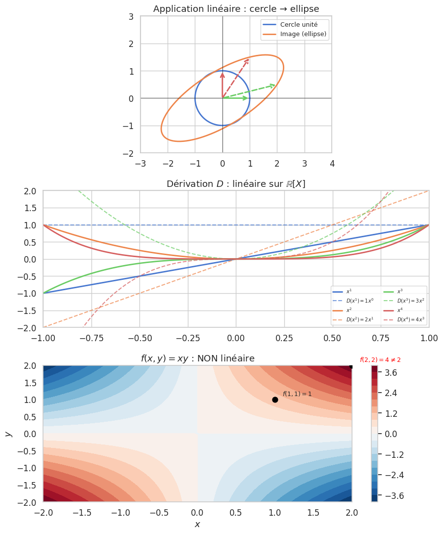
\((x,y) \mapsto (x+y, x-y)\) sur \(\mathbb{R}^2\)	Oui	Matrice \(\begin{pmatrix}1&1\\1&-1\end{pmatrix}\)
\(x \mapsto x + 1\) sur \(\mathbb{R}\)	Non	\(f(0) = 1 \neq 0\)
\(f \mapsto f'\) sur \(\mathcal{C}^1(I)\)	Oui	Dérivation
\(f \mapsto \int_a^b f\) sur \(\mathcal{C}^0([a,b])\)	Oui	Forme linéaire
\((x,y) \mapsto xy\) sur \(\mathbb{R}^2\)	Non	Pas homogène
Projection sur \(F\) parallèlement à \(G\)	Oui	Si \(E = F \oplus G\)

Show code cell source

Hide code cell source

import numpy as np
import matplotlib.pyplot as plt
import seaborn as sns

sns.set_theme(style="whitegrid", palette="muted", font_scale=1.1)

fig, axes = plt.subplots(3, 1, figsize=(9, 11))

# 1. Transformation linéaire : cercle -> ellipse
theta = np.linspace(0, 2*np.pi, 200)
circle = np.vstack([np.cos(theta), np.sin(theta)])

A = np.array([[2, 1], [0.5, 1.5]])
ellipse = A @ circle

ax = axes[0]
ax.plot(circle[0], circle[1], 'C0-', lw=2, label='Cercle unité')
ax.plot(ellipse[0], ellipse[1], 'C1-', lw=2, label='Image (ellipse)')
ax.axhline(0, color='k', lw=0.5); ax.axvline(0, color='k', lw=0.5)
# Vecteurs de base et leurs images
for e, c in [(np.array([1,0]),'C2'), (np.array([0,1]),'C3')]:
    ax.annotate('', xy=e, xytext=(0,0), arrowprops=dict(arrowstyle='->', color=c, lw=2))
    fe = A @ e
    ax.annotate('', xy=fe, xytext=(0,0), arrowprops=dict(arrowstyle='->', color=c, lw=2, ls='--'))
ax.set(aspect='equal', title='Application linéaire : cercle → ellipse', xlim=(-3,4), ylim=(-2,3))
ax.legend(fontsize=9)

# 2. Dérivation sur les polynômes : D(x^k) = k x^{k-1}
x = np.linspace(-1, 1, 200)
ax2 = axes[1]
for k, col in [(1,'C0'),(2,'C1'),(3,'C2'),(4,'C3')]:
    ax2.plot(x, x**k, col+'-', lw=2, label=f'$x^{k}$')
    ax2.plot(x, k*x**(k-1) if k > 0 else np.zeros_like(x),
             col+'--', lw=1.5, alpha=0.7, label=f"$D(x^{k}) = {k}x^{k-1}$")
ax2.set(xlim=(-1,1), ylim=(-2,2), title='Dérivation $D$ : linéaire sur $\\mathbb{R}[X]$')
ax2.legend(fontsize=7, ncol=2)

# 3. Application non-linéaire : f(x,y) = x*y
from matplotlib.colors import Normalize
x_vals = np.linspace(-2, 2, 50)
y_vals = np.linspace(-2, 2, 50)
X, Y = np.meshgrid(x_vals, y_vals)
Z = X * Y  # Non-linéaire
im = axes[2].contourf(X, Y, Z, levels=20, cmap='RdBu_r')
plt.colorbar(im, ax=axes[2])
axes[2].set(xlabel='$x$', ylabel='$y$', title='$f(x,y)=xy$ : NON linéaire')
# Montrer f(2*(1,1)) ≠ 2*f(1,1)
axes[2].scatter([1,2], [1,2], color='black', s=60, zorder=5)
axes[2].text(1.1, 1.1, '$f(1,1)=1$', fontsize=9)
axes[2].text(2.1, 2.1, '$f(2,2)=4 \\neq 2$', fontsize=9, color='red')

plt.tight_layout()
plt.show()

Structure de \(\mathcal{L}(E, F)\)

Proposition 227 (\(\mathcal{L}(E, F)\) est un espace vectoriel)

\((f+g)(u) = f(u)+g(u)\) et \((\lambda f)(u) = \lambda f(u)\) munissent \(\mathcal{L}(E,F)\) d’une structure de \(\mathbb{K}\)-ev.

Proposition 228 (Composition et algèbre)

Si \(f \in \mathcal{L}(E,F)\) et \(g \in \mathcal{L}(F,G)\), alors \(g \circ f \in \mathcal{L}(E,G)\).

\((\mathcal{L}(E), +, \circ)\) est un anneau (non commutatif pour \(\dim E \geq 2\)) d’élément neutre \(\mathrm{id}_E\).

Proposition 229 (Dimension de \(\mathcal{L}(E, F)\))

Si \(\dim E = n\) et \(\dim F = p\) : \(\dim \mathcal{L}(E, F) = np\).

Proof. L’application \(\Phi : f \mapsto \text{Mat}(f)\) (matrice dans des bases fixées) est un isomorphisme \(\mathcal{L}(E,F) \xrightarrow{\sim} \mathcal{M}_{p,n}(\mathbb{K})\), qui est de dimension \(pn\).

Image, noyau, rang

Définition 146 (Noyau et image)

Pour \(f \in \mathcal{L}(E,F)\) :

\[\ker f = \{u \in E \mid f(u) = 0_F\}, \qquad \mathrm{Im}\, f = \{f(u) \mid u \in E\}.\]

\(\ker f\) est un sev de \(E\) et \(\mathrm{Im}\, f\) est un sev de \(F\).

Proof. Noyau. \(0_E \in \ker f\). Si \(u, v \in \ker f\) : \(f(\lambda u + v) = \lambda f(u) + f(v) = 0\). ✓

Image. \(0_F = f(0_E) \in \mathrm{Im}\, f\). Si \(w_i = f(u_i) \in \mathrm{Im}\, f\) : \(\lambda w_1 + w_2 = f(\lambda u_1 + u_2) \in \mathrm{Im}\, f\). ✓

Proposition 230 (Injectivité et noyau)

\[f \text{ injective} \iff \ker f = \{0_E\}.\]

Proof. \((\Rightarrow)\) Si \(f(u) = 0 = f(0)\), alors \(u = 0\) par injectivité. \((\Leftarrow)\) Si \(f(u) = f(v)\), alors \(f(u-v) = 0\), donc \(u-v \in \ker f = \{0\}\).

Définition 147 (Rang)

Le rang de \(f\) est \(\mathrm{rg}\, f = \dim(\mathrm{Im}\, f)\).

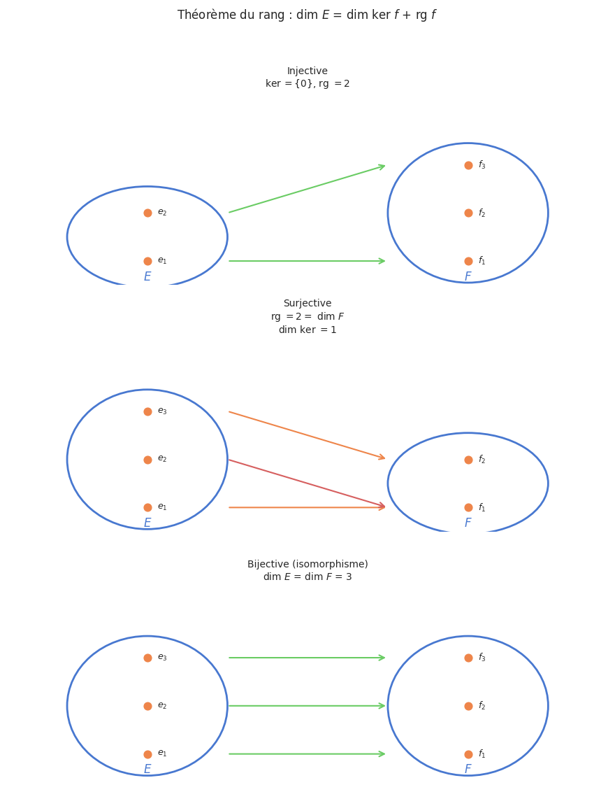
Proposition 231 (Théorème du rang)

\[\dim E = \dim(\ker f) + \mathrm{rg}\, f.\]

Proof. Soit \((e_1, \ldots, e_r)\) base de \(\ker f\), complétée en base \((e_1,\ldots,e_r, e_{r+1},\ldots,e_n)\) de \(E\).

\((f(e_{r+1}), \ldots, f(e_n))\) est une base de \(\mathrm{Im}\, f\).

Génératrice. Pour tout \(u = \sum \lambda_i e_i\), \(f(u) = \sum_{i>r} \lambda_i f(e_i)\) (car \(f(e_i)=0\) pour \(i\leq r\)). ✓

Libre. Si \(\sum_{i>r} \lambda_i f(e_i) = 0\), alors \(f(\sum_{i>r}\lambda_i e_i) = 0\), donc \(\sum_{i>r}\lambda_i e_i \in \ker f = \mathrm{Vect}(e_1,\ldots,e_r)\). Comme \((e_1,\ldots,e_n)\) est libre : \(\lambda_i = 0\). ✓

Donc \(\mathrm{rg}\, f = n - r\).

Proposition 232 (Corollaires du théorème du rang)

Soit \(f \in \mathcal{L}(E,F)\) avec \(\dim E = n\), \(\dim F = p\).

Propriété	Condition
\(f\) injective	\(\ker f = \{0\}\), i.e. \(\mathrm{rg}\, f = n\)
\(f\) surjective	\(\mathrm{Im}\, f = F\), i.e. \(\mathrm{rg}\, f = p\)
\(f\) bijective (isomorphisme)	\(\mathrm{rg}\, f = n = p\)
Borne sur le rang	\(\mathrm{rg}\, f \leq \min(n,p)\)

En dimension finie égale (\(n = p\)) : injective \(\iff\) surjective \(\iff\) bijective.

Show code cell source

Hide code cell source

fig, axes = plt.subplots(3, 1, figsize=(9, 11))

def draw_mapping(ax, dom_pts, cod_pts, arrows, title, dom_name='$E$', cod_name='$F$'):
    """Dessine une application avec points et flèches."""
    ax.axis('off')
    ax.set_xlim(0, 3); ax.set_ylim(-0.5, len(max(dom_pts, cod_pts, key=len))+0.5)
    # Ellipses
    from matplotlib.patches import Ellipse
    for cx, pts, name in [(0.7, dom_pts, dom_name), (2.3, cod_pts, cod_name)]:
        h = max(len(pts), 2) * 0.8 + 0.5
        ell = Ellipse((cx, (len(pts)-1)/2), 0.8, h, fill=False, color='C0', lw=2)
        ax.add_patch(ell)
        ax.text(cx, -0.4, name, ha='center', fontsize=12, color='C0')
        for i, p in enumerate(pts):
            ax.scatter([cx], [i], s=60, color='C1', zorder=5)
            ax.text(cx+0.05, i, p, fontsize=9, va='center')
    for (i, j, c) in arrows:
        ax.annotate('', xy=(1.9, j), xytext=(1.1, i),
                    arrowprops=dict(arrowstyle='->', color=c, lw=1.5))
    ax.set_title(title, fontsize=10)

# Injection : ker = {0}, rg = dim E < dim F
draw_mapping(axes[0],
    ['$e_1$', '$e_2$'],
    ['$f_1$', '$f_2$', '$f_3$'],
    [(0, 0, 'C2'), (1, 2, 'C2')],
    'Injective\n$\\ker = \\{0\\}$, rg $= 2$')

# Surjection : rg = dim F < dim E
draw_mapping(axes[1],
    ['$e_1$', '$e_2$', '$e_3$'],
    ['$f_1$', '$f_2$'],
    [(0, 0, 'C1'), (1, 0, 'C3'), (2, 1, 'C1')],
    'Surjective\nrg $= 2 =$ dim $F$\ndim ker $= 1$')

# Bijection
draw_mapping(axes[2],
    ['$e_1$', '$e_2$', '$e_3$'],
    ['$f_1$', '$f_2$', '$f_3$'],
    [(0, 0, 'C2'), (1, 1, 'C2'), (2, 2, 'C2')],
    'Bijective (isomorphisme)\ndim $E$ = dim $F$ = 3')

plt.suptitle('Théorème du rang : dim $E$ = dim ker $f$ + rg $f$', fontsize=12, y=1.02)
plt.tight_layout()
plt.show()

Détermination par l’image d’une base

Proposition 233 (Théorème de détermination)

Soit \((e_1, \ldots, e_n)\) une base de \(E\) et \(w_1, \ldots, w_n \in F\) quelconques. Il existe une unique \(f \in \mathcal{L}(E,F)\) telle que \(f(e_i) = w_i\) pour tout \(i\).

Proof. Existence. \(f\!\left(\sum \lambda_i e_i\right) = \sum \lambda_i w_i\) est bien définie (coordonnées uniques) et linéaire. ✓

Unicité. Si \(g \in \mathcal{L}(E,F)\) vérifie \(g(e_i) = w_i\), alors pour tout \(u = \sum\lambda_i e_i\) : \(g(u) = \sum \lambda_i w_i = f(u)\). ✓

Remarque 88

Ce théorème est fondamental : pour définir une application linéaire sur \(E\), il suffit de choisir librement les images des vecteurs d’une base. C’est ainsi que l’on construit tous les isomorphismes.

Proposition 234 (Isomorphisme et dimension)

\(E \simeq F \iff \dim E = \dim F\).

En particulier, tout ev de dimension \(n\) est isomorphe à \(\mathbb{K}^n\).

Projecteurs et symétries

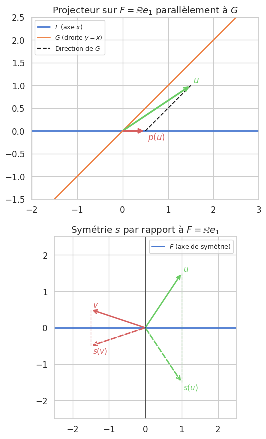
Définition 148 (Projecteur)

Soit \(E = F \oplus G\). Le projecteur sur \(F\) parallèlement à \(G\) est

\[p : u = u_F + u_G \mapsto u_F.\]

Proposition 235 (Caractérisation des projecteurs)

\(p \in \mathcal{L}(E)\) est un projecteur \(\iff\) \(p^2 = p\) (idempotent).

Dans ce cas : \(\mathrm{Im}\, p = \ker(p - \mathrm{id})\) et \(\ker p = \mathrm{Im}(\mathrm{id} - p)\), avec \(E = \mathrm{Im}\, p \oplus \ker p\).

Proof. \((\Rightarrow)\) Si \(u = u_F + u_G\) : \(p^2(u) = p(u_F) = u_F = p(u)\) (car \(u_F \in F\)). ✓

\((\Leftarrow)\) Pour \(u \in E\) : \(u = p(u) + (u - p(u))\). On a \(p(u) \in \mathrm{Im}\, p\) et \(p(u - p(u)) = p(u) - p^2(u) = 0\), donc \(u - p(u) \in \ker p\). Si \(v \in \mathrm{Im}\, p \cap \ker p\) : \(v = p(w)\) et \(p(v) = 0\), d’où \(v = p^2(w) = p(v) = 0\).

Définition 149 (Symétrie)

La symétrie par rapport à \(F\) parallèlement à \(G\) est \(s = 2p - \mathrm{id}\) :

\[s(u_F + u_G) = u_F - u_G.\]

\(s\) est une involution : \(s^2 = \mathrm{id}\). Valeurs propres : \(+1\) (sur \(F\)) et \(-1\) (sur \(G\)).

Show code cell source

Hide code cell source

fig, axes = plt.subplots(2, 1, figsize=(9, 9))

# Projecteur dans R^2 : proj sur axe x parallèlement à une droite oblique
ax = axes[0]
ax.set(xlim=(-2, 3), ylim=(-1.5, 2.5), aspect='equal',
       title='Projecteur sur $F=\\mathbb{R}e_1$ parallèlement à $G$')
ax.axhline(0, color='C0', lw=2, label='$F$ (axe $x$)')
# Direction de G : (1, 1)
t = np.linspace(-1.5, 2.5, 100)
ax.plot(t, t, 'C1-', lw=2, label='$G$ (droite $y=x$)')
# Vecteur u et sa projection
u = np.array([1.5, 1.0])
ax.annotate('', xy=u, xytext=(0,0), arrowprops=dict(arrowstyle='->', color='C2', lw=2.5))
ax.text(u[0]+0.05, u[1]+0.05, '$u$', fontsize=12, color='C2')
# Projection : sur axe x, parallèlement à (1,1) => retirer la composante sur G
# Si G = Vect(1,1) et F = axe x, alors p(a,b) = (a-b, 0)
pu = np.array([u[0]-u[1], 0])
ax.annotate('', xy=pu, xytext=(0,0), arrowprops=dict(arrowstyle='->', color='C3', lw=2.5))
ax.text(pu[0]+0.05, pu[1]-0.2, '$p(u)$', fontsize=12, color='C3')
ax.plot([u[0], pu[0]], [u[1], pu[1]], 'k--', lw=1.5, label='Direction de $G$')
ax.axhline(0, color='k', lw=0.5); ax.axvline(0, color='k', lw=0.5)
ax.legend(fontsize=9)

# Symétrie dans R^2 : s par rapport à l'axe x
ax2 = axes[1]
ax2.set(xlim=(-2.5, 2.5), ylim=(-2.5, 2.5), aspect='equal',
        title='Symétrie $s$ par rapport à $F=\\mathbb{R}e_1$')
ax2.axhline(0, color='C0', lw=2, label='$F$ (axe de symétrie)')
ax2.axvline(0, color='k', lw=0.5)
for u, c, lbl in [(np.array([1, 1.5]), 'C2', '$u$'), (np.array([-1.5, 0.5]), 'C3', '$v$')]:
    su = np.array([u[0], -u[1]])
    ax2.annotate('', xy=u, xytext=(0,0), arrowprops=dict(arrowstyle='->', color=c, lw=2))
    ax2.annotate('', xy=su, xytext=(0,0), arrowprops=dict(arrowstyle='->', color=c, lw=2, ls='--'))
    ax2.text(u[0]+0.05, u[1]+0.05, lbl, fontsize=11, color=c)
    ax2.text(su[0]+0.05, su[1]-0.2, f'$s({lbl[1:-1]})$', fontsize=11, color=c)
    ax2.plot([u[0], su[0]], [u[1], su[1]], '--', color=c, lw=1, alpha=0.5)
ax2.legend(fontsize=9)

plt.tight_layout()
plt.show()

Formes linéaires et hyperplans

Définition 150 (Hyperplan)

Un hyperplan de \(E\) est un sev de dimension \(\dim E - 1\), i.e. le noyau d’une forme linéaire non nulle.

\[H = \ker \varphi = \{u \in E \mid \varphi(u) = 0\}, \quad \varphi \in E^* \setminus \{0\}.\]

Exemple 81

• Dans \(\mathbb{R}^3\) : les plans passant par l’origine \(ax + by + cz = 0\) sont les hyperplans.

• Dans \(\mathbb{R}^n\) : \(H = \{(x_1,\ldots,x_n) \mid \sum a_i x_i = 0\}\).

• \(\ker D\) (polynômes de dérivée nulle) = polynômes constants dans \(\mathbb{R}_n[X]\).

Proposition 236

Deux formes linéaires \(\varphi, \psi \in E^*\) ont même noyau \(\iff\) elles sont proportionnelles : \(\psi = \lambda \varphi\) pour un \(\lambda \in \mathbb{K}\).

Proof. \((\Leftarrow)\) Immédiat. \((\Rightarrow)\) Soit \(u_0 \notin H = \ker\varphi\). Tout \(u \in E\) s’écrit \(u = \lambda u_0 + v\) avec \(v \in H\) (car \(E = \mathbb{K}u_0 \oplus H\)). Alors \(\varphi(u) = \lambda\varphi(u_0)\) et \(\psi(u) = \lambda\psi(u_0)\). D’où \(\psi = \frac{\psi(u_0)}{\varphi(u_0)}\varphi\).

Endomorphismes remarquables

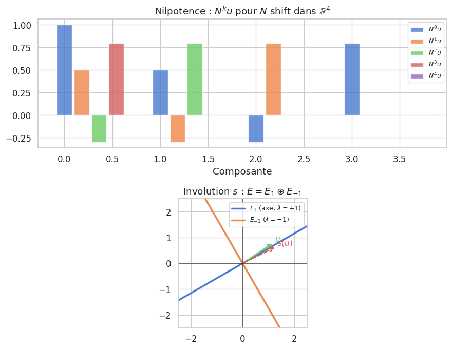
Définition 151 (Nilpotent)

\(f \in \mathcal{L}(E)\) est nilpotent d’indice \(k\) si \(f^k = 0\) et \(f^{k-1} \neq 0\).

Propriété clé. Si \(f\) est nilpotent d’indice \(k\) sur un ev de dimension \(n\), alors \(k \leq n\).

Proof. La chaîne \(E \supset \mathrm{Im}\, f \supset \mathrm{Im}\, f^2 \supset \cdots \supset \mathrm{Im}\, f^k = \{0\}\) est strictement décroissante (jusqu’à l’indice \(k\)), donc chaque inclusion diminue la dimension d’au moins 1. Ainsi \(k \leq n\).

Exemple 82

Sur \(\mathbb{R}_n[X]\), la dérivation \(D\) est nilpotente d’indice \(n+1\) : \(D^{n+1} = 0\).

La matrice \(N = \begin{pmatrix} 0 & 1 & 0 \\ 0 & 0 & 1 \\ 0 & 0 & 0 \end{pmatrix}\) est nilpotente d’indice 3 : \(N^2 \neq 0\), \(N^3 = 0\).

Définition 152 (Involution)

\(f\) est une involution si \(f^2 = \mathrm{id}\).

Caractérisation. \(f\) est une involution \(\iff\) \(f\) est une symétrie. Dans ce cas : \(E = E_1 \oplus E_{-1}\) (valeurs propres \(\pm 1\)), où \(E_{\pm 1} = \ker(f \mp \mathrm{id})\).

Show code cell source

Hide code cell source

fig, axes = plt.subplots(2, 1, figsize=(9, 7))

# Nilpotence : dim Im f^k décroit
# Illustration sur R^4, application shift : (x1,x2,x3,x4) -> (0,x1,x2,x3)
N4 = np.diag([1,1,1], k=1)  # shift
u = np.random.seed(0); u = np.array([1.0, 0.5, -0.3, 0.8])
powers = [u]
v = u.copy()
for _ in range(4):
    v = N4 @ v
    powers.append(v.copy())

ax = axes[0]
x = np.arange(4)
for i, p in enumerate(powers):
    ax.bar(x + i*0.18, p, width=0.16, label=f'$N^{i}u$', alpha=0.8)
ax.set(xlabel='Composante', title='Nilpotence : $N^k u$ pour $N$ shift dans $\\mathbb{R}^4$')
ax.legend(fontsize=9)

# Décomposition E = E_1 ⊕ E_{-1} pour une involution (symétrie)
ax2 = axes[1]
ax2.set(xlim=(-2.5, 2.5), ylim=(-2.5, 2.5), aspect='equal',
        title='Involution $s$ : $E = E_1 \\oplus E_{-1}$')
# Axe de symétrie (E_1) et direction inverse (E_{-1})
t = np.linspace(-2.5, 2.5, 100)
ax2.plot(t, t*np.tan(np.pi/6), 'C0-', lw=2.5, label='$E_1$ (axe, $\\lambda=+1$)')
ax2.plot(t, -t/np.tan(np.pi/6), 'C1-', lw=2.5, label='$E_{-1}$ ($\\lambda=-1$)')
ax2.axhline(0, color='k', lw=0.4); ax2.axvline(0, color='k', lw=0.4)
# Exemple de vecteur et son image
u2 = np.array([1.2, 0.8])
angle = np.pi/6
# Symétrie par rapport à la droite y = x*tan(angle)
cos2, sin2 = np.cos(2*angle), np.sin(2*angle)
su2 = np.array([cos2*u2[0]+sin2*u2[1], sin2*u2[0]-cos2*u2[1]])
ax2.annotate('', xy=u2, xytext=(0,0), arrowprops=dict(arrowstyle='->', color='C2', lw=2))
ax2.annotate('', xy=su2, xytext=(0,0), arrowprops=dict(arrowstyle='->', color='C3', lw=2, ls='--'))
ax2.text(u2[0]+0.05, u2[1]+0.05, '$u$', fontsize=11, color='C2')
ax2.text(su2[0]+0.05, su2[1]+0.05, '$s(u)$', fontsize=11, color='C3')
ax2.legend(fontsize=9)

plt.tight_layout()
plt.show()

Théorèmes d’isomorphisme

Proposition 237 (Premier théorème d’isomorphisme)

Soit \(f \in \mathcal{L}(E, F)\). L’application \(\bar{f} : E/\ker f \to \mathrm{Im}\, f\) définie par \(\bar{f}(u + \ker f) = f(u)\) est un isomorphisme :

\[E / \ker f \simeq \mathrm{Im}\, f.\]

En particulier, \(\dim(E/\ker f) = \mathrm{rg}\, f\).

Proof. \(\bar{f}\) est bien définie (si \(u - v \in \ker f\), \(f(u) = f(v)\)), linéaire, injective (si \(\bar{f}(u+\ker f) = 0\), \(u \in \ker f\)), et surjective sur \(\mathrm{Im}\, f\).

Remarque 89

L’espace quotient \(E/\ker f\) est l’espace des classes \(u + \ker f = \{u + v \mid v \in \ker f\}\). C’est l’analogue vectoriel du théorème d’isomorphisme des groupes (\(G/\ker\phi \simeq \mathrm{Im}\,\phi\), cf. chapitre 03).