Le corps \(\mathbb{C}\) des complexes

Les nombres imaginaires sont une magnifique et merveilleuse ressource de l’esprit divin, presque un amphibie entre l’être et le non-être.

Gottfried Wilhelm Leibniz

Construction et structure algébrique

Définition 60 (L’ensemble \(\mathbb{C}\))

\(\mathbb{C} = \mathbb{R}^2\) muni de l’addition \((a,b) + (c,d) = (a+c, b+d)\) et de la multiplication

\[(a, b) \cdot (c, d) = (ac - bd,\ ad + bc)\]

Proposition 74 (\((\mathbb{C}, +, \cdot)\) est un corps commutatif)

L’unité imaginaire \(i = (0, 1)\) vérifie \(i^2 = -1\). Tout complexe s’écrit \(z = a + ib\) (forme algébrique) avec \(a = \text{Re}(z)\), \(b = \text{Im}(z)\). L’inverse de \(z \neq 0\) est \(z^{-1} = \frac{\bar{z}}{|z|^2}\).

Remarque 31

\(\mathbb{C}\) n’est pas ordonnable : si \(i > 0\), alors \(i^2 = -1 > 0\), contradiction. Si \(i < 0\), alors \(-i > 0\), donc \((-i)^2 = -1 > 0\), même contradiction.

Conjugaison et module

Définition 61 (Conjugué et module)

Pour \(z = a + ib\) :

• Conjugué : \(\bar{z} = a - ib\)

• Module : \(|z| = \sqrt{a^2 + b^2} = \sqrt{z\bar{z}}\)

Proposition 75 (Propriétés)

\(\overline{z + w} = \bar{z} + \bar{w}\), \(\overline{zw} = \bar{z}\bar{w}\), \(\overline{\bar{z}} = z\).

\(|zw| = |z||w|\), \(|z + w| \leq |z| + |w|\), \(\big||z| - |w|\big| \leq |z - w|\).

\(\text{Re}(z) = \frac{z + \bar{z}}{2}\), \(\text{Im}(z) = \frac{z - \bar{z}}{2i}\).

Proof. \(|z+w|^2 = (z+w)\overline{(z+w)} = |z|^2 + z\bar{w} + \bar{z}w + |w|^2 = |z|^2 + 2\text{Re}(z\bar{w}) + |w|^2 \leq |z|^2 + 2|z||w| + |w|^2 = (|z|+|w|)^2\).

Forme trigonométrique et exponentielle complexe

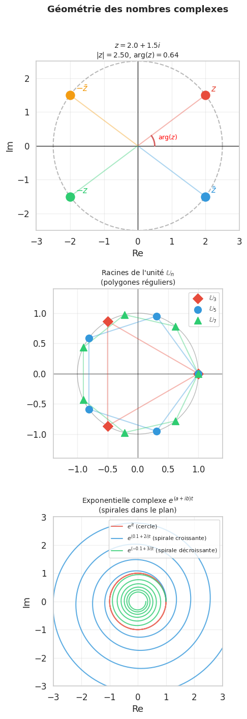
Définition 62 (Argument et forme trigonométrique)

Pour \(z \neq 0\), l”argument \(\theta = \arg(z)\) est l’angle \(\theta \in \: ]-\pi, \pi]\) tel que \(z = |z|(\cos\theta + i\sin\theta)\).

La forme exponentielle est \(z = |z|e^{i\theta}\), où \(e^{i\theta} = \cos\theta + i\sin\theta\) (formule d’Euler).

Proposition 76 (Formule de Moivre et multiplication)

\((r_1 e^{i\theta_1})(r_2 e^{i\theta_2}) = r_1 r_2 e^{i(\theta_1 + \theta_2)}\)

\[(\cos\theta + i\sin\theta)^n = \cos(n\theta) + i\sin(n\theta) \quad \forall n \in \mathbb{Z}\]

Proof. Par récurrence pour \(n \geq 0\), en utilisant la formule d’addition trigonométrique. Pour \(n < 0\), utiliser \((\cos\theta + i\sin\theta)^{-1} = \cos(-\theta) + i\sin(-\theta)\).

Exemple 24

Linéarisation de \(\cos^3\theta\) : \(\cos^3\theta = \left(\frac{e^{i\theta}+e^{-i\theta}}{2}\right)^3 = \frac{e^{3i\theta}+3e^{i\theta}+3e^{-i\theta}+e^{-3i\theta}}{8} = \frac{\cos3\theta + 3\cos\theta}{4}\)

Formules de Moivre pour \(\cos(3\theta)\) : \((\cos\theta+i\sin\theta)^3 = \cos^3\theta - 3\cos\theta\sin^2\theta + i(3\cos^2\theta\sin\theta - \sin^3\theta)\)

Donc \(\cos(3\theta) = 4\cos^3\theta - 3\cos\theta\) et \(\sin(3\theta) = 3\sin\theta - 4\sin^3\theta\).

Proposition 77 (Identité d’Euler)

\[e^{i\pi} + 1 = 0\]

Cette identité relie les cinq constantes fondamentales : \(0\), \(1\), \(e\), \(i\), \(\pi\).

Logarithme complexe et exponentielle

Définition 63 (Exponentielle complexe)

Pour \(z = x + iy\) :

\[e^z = e^x(\cos y + i\sin y)\]

Proposition 78 (Propriétés de l’exponentielle complexe)

• \(e^{z+w} = e^z e^w\)

• \(|e^z| = e^{\text{Re}(z)}\)

• \(e^z = 1 \iff z \in 2i\pi\mathbb{Z}\)

• La fonction \(z \mapsto e^z\) est \(2i\pi\)-périodique

• \(\frac{d}{dz} e^z = e^z\)

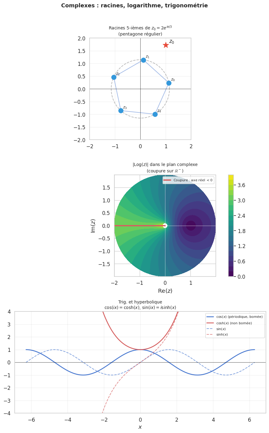
Définition 64 (Logarithme complexe)

Le logarithme principal est défini pour \(z \notin \mathbb{R}^-\) par :

\[\text{Log}(z) = \ln|z| + i\arg(z), \quad \arg(z) \in \: ]-\pi, \pi[\]

Remarque 32

Le logarithme complexe est multivalué : si \(e^w = z\), alors \(e^{w + 2ik\pi} = z\) pour tout \(k \in \mathbb{Z}\).

Toutes les valeurs : \(\log(z) = \ln|z| + i(\arg(z) + 2k\pi)\), \(k \in \mathbb{Z}\).

Par exemple : \(\text{Log}(-1) = i\pi\), \(\log(-1) = i\pi(2k+1)\), \(k \in \mathbb{Z}\).

Exemple 25

Puissances complexes : On peut définir \(z^w = e^{w \text{Log}(z)}\) (choix de branche).

\(i^i = e^{i \text{Log}(i)} = e^{i \cdot i\pi/2} = e^{-\pi/2} \approx 0.2079\ldots\) (réel !)

\((-1)^{\sqrt{2}} = e^{\sqrt{2}\, i\pi}\) est complexe non réel.

Racines \(n\)-ièmes

Proposition 79 (Racines \(n\)-ièmes d’un complexe)

Soit \(z_0 = r_0 e^{i\theta_0} \neq 0\) et \(n \in \mathbb{N}^*\). L’équation \(z^n = z_0\) admet exactement \(n\) solutions :

\[z_k = r_0^{1/n} \exp\!\left(i\frac{\theta_0 + 2k\pi}{n}\right), \quad k = 0, 1, \ldots, n-1\]

Elles forment les sommets d’un polygone régulier à \(n\) côtés inscrit dans le cercle de rayon \(r_0^{1/n}\).

Proof. Si \(z = \rho e^{i\varphi}\), \(z^n = z_0 \iff \rho^n = r_0 \land n\varphi = \theta_0 + 2k\pi\). Donc \(\rho = r_0^{1/n}\) (unique) et \(\varphi = \frac{\theta_0 + 2k\pi}{n}\). Les valeurs distinctes sont pour \(k = 0, \ldots, n-1\) (les autres se répètent par \(2\pi\)-périodicité).

Définition 65 (Racines \(n\)-ièmes de l’unité)

Les racines \(n\)-ièmes de l’unité sont \(\mathbb{U}_n = \{e^{2ik\pi/n} \mid k = 0, \ldots, n-1\}\).

\((\mathbb{U}_n, \cdot)\) est un groupe cyclique d’ordre \(n\), engendré par \(\omega_n = e^{2i\pi/n}\) (racine primitive).

Proposition 80 (Somme des racines de l’unité)

\(\displaystyle\sum_{k=0}^{n-1} e^{2ik\pi/n} = 0\) pour \(n \geq 2\).

Plus généralement : \(\displaystyle\sum_{k=0}^{n-1} e^{2ijk\pi/n} = \begin{cases} n & \text{si } n \mid j \\ 0 & \text{sinon} \end{cases}\)

Proof. \(\sum_{k=0}^{n-1} \omega^k = \frac{\omega^n - 1}{\omega - 1} = \frac{1 - 1}{\omega - 1} = 0\) pour \(\omega = e^{2i\pi/n} \neq 1\).

La formule générale utilise \(\sum_{k=0}^{n-1} (e^{2ij\pi/n})^k\).

Exemple 26

Résoudre \(z^4 + 1 = 0\) : \(z^4 = -1 = e^{i\pi}\). Les solutions sont \(e^{i(\pi/4 + k\pi/2)}\) pour \(k = 0, 1, 2, 3\), soit \(\frac{\pm 1 \pm i}{\sqrt{2}}\).

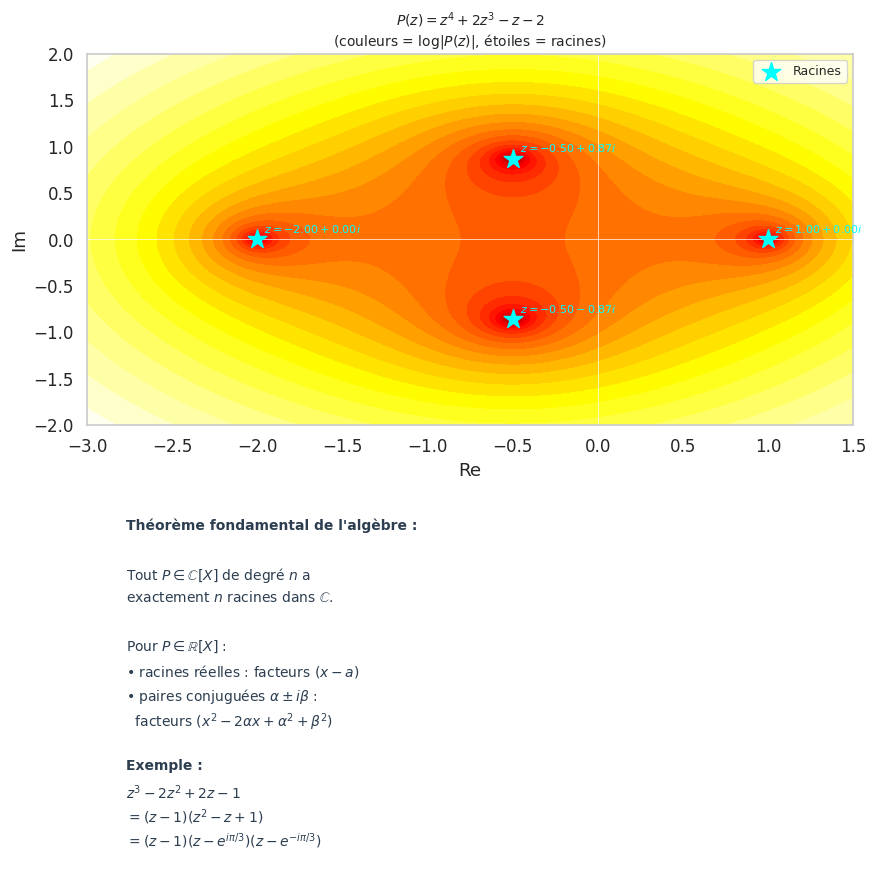
Théorème fondamental de l’algèbre

Proposition 81 (Théorème de d’Alembert-Gauss)

Tout polynôme non constant à coefficients complexes admet au moins une racine dans \(\mathbb{C}\).

Corollaire : tout polynôme de degré \(n\) à coefficients complexes admet exactement \(n\) racines dans \(\mathbb{C}\) (comptées avec multiplicité).

Remarque 33

\(\mathbb{C}\) est algébriquement clos : c’est la « clôture algébrique » de \(\mathbb{R}\). Il n’y a pas d’extension algébrique propre de \(\mathbb{C}\).

Conséquence pour les polynômes réels : les racines complexes non réelles viennent par paires conjuguées \(z\) et \(\bar{z}\). Donc tout polynôme réel se factorise en facteurs de degré 1 (racines réelles) et de degré 2 (paires conjuguées) dans \(\mathbb{R}[X]\).

Trigonométrie complexe

Définition 66 (Fonctions trigonométriques et hyperboliques via \(\mathbb{C}\))

\[\cos z = \frac{e^{iz} + e^{-iz}}{2}, \quad \sin z = \frac{e^{iz} - e^{-iz}}{2i}\]

\[\cosh z = \frac{e^z + e^{-z}}{2} = \cos(iz), \quad \sinh z = \frac{e^z - e^{-z}}{2} = -i\sin(iz)\]

Proposition 82 (Relations entre trigonométrie complexe et hyperbolique)

\[\cos(iz) = \cosh z, \quad \sin(iz) = i\sinh z\]

\[\cosh(iz) = \cos z, \quad \sinh(iz) = i\sin z\]

Ces relations (règle d’Osborn) permettent de passer des formules trigonométriques aux formules hyperboliques en remplaçant \(\sin\) par \(i\sinh\) (et \(\cos\) par \(\cosh\)).

Proposition 83 (Formule de Moivre généralisée et linéarisation)

Grâce à \(e^{i\theta} = \cos\theta + i\sin\theta\) et \(e^{-i\theta} = \cos\theta - i\sin\theta\) :

\[\begin{split}\cos^n\theta = \frac{1}{2^n}\sum_{k=0}^{n} \binom{n}{k} e^{i(2k-n)\theta} = \frac{1}{2^{n-1}} \cdot \begin{cases} \sum_{k=0}^{(n-1)/2} \binom{n}{k}\cos((n-2k)\theta) & n \text{ impair} \\ \frac{1}{2}\binom{n}{n/2} + \sum_{k=0}^{n/2-1}\binom{n}{k}\cos((n-2k)\theta) & n \text{ pair} \end{cases}\end{split}\]

Show code cell source

Hide code cell source

import numpy as np
import matplotlib.pyplot as plt
import seaborn as sns

sns.set_theme(style="whitegrid", palette="muted", font_scale=1.1)

Show code cell source

Hide code cell source

# Plan complexe : module, argument, conjugaison
fig, axes = plt.subplots(3, 1, figsize=(9, 14))

theta_circle = np.linspace(0, 2 * np.pi, 300)

# --- Plan complexe avec z, z_bar, -z, -z_bar ---
ax = axes[0]
z = 2 + 1.5j
z_bar = np.conj(z)
points = {'$z$': z, '$\\bar{z}$': z_bar, '$-z$': -z, '$-\\bar{z}$': -z_bar}
colors_pts = {'$z$': '#e74c3c', '$\\bar{z}$': '#3498db', '$-z$': '#2ecc71', '$-\\bar{z}$': '#f39c12'}

ax.plot(np.cos(theta_circle) * abs(z), np.sin(theta_circle) * abs(z), 'k--', alpha=0.3)
ax.axhline(0, color='black', lw=0.8); ax.axvline(0, color='black', lw=0.8)

for label, pt in points.items():
    ax.scatter([pt.real], [pt.imag], s=150, color=colors_pts[label], zorder=5)
    ax.annotate(label, (pt.real, pt.imag), textcoords='offset points',
               xytext=(8, 5), fontsize=12, color=colors_pts[label])
    ax.plot([0, pt.real], [0, pt.imag], color=colors_pts[label], alpha=0.4, lw=1.5)

# Arc d'argument
theta_arc = np.linspace(0, np.angle(z), 50)
r_arc = 0.5
ax.plot(r_arc * np.cos(theta_arc), r_arc * np.sin(theta_arc), 'r-', lw=2)
ax.text(0.6, 0.2, f'$\\arg(z)$', fontsize=9, color='red')

ax.set_xlim(-3, 3); ax.set_ylim(-2.5, 2.5)
ax.set_aspect('equal')
ax.set_xlabel('Re'); ax.set_ylabel('Im')
ax.set_title(f'$z = {z.real}+{z.imag}i$\n$|z|={abs(z):.2f}$, $\\arg(z)={np.angle(z):.2f}$', fontsize=10)
ax.grid(True, alpha=0.3)

# --- Racines n-ièmes de l'unité ---
ax2 = axes[1]
ax2.plot(np.cos(theta_circle), np.sin(theta_circle), 'k-', alpha=0.3, lw=1)
ax2.axhline(0, color='black', lw=0.5); ax2.axvline(0, color='black', lw=0.5)

for n_roots, color, marker in [(3, '#e74c3c', 'D'), (5, '#3498db', 'o'), (7, '#2ecc71', '^')]:
    angles_roots = np.linspace(0, 2 * np.pi, n_roots, endpoint=False)
    xs = np.cos(angles_roots); ys = np.sin(angles_roots)
    ax2.scatter(xs, ys, s=100, color=color, marker=marker, zorder=5,
               label=f'$\\mathbb{{U}}_{n_roots}$')
    # Polygone
    ax2.plot(np.append(xs, xs[0]), np.append(ys, ys[0]), color=color, alpha=0.4, lw=1.5)

ax2.set_xlim(-1.4, 1.4); ax2.set_ylim(-1.4, 1.4)
ax2.set_aspect('equal')
ax2.set_title('Racines de l\'unité $\\mathbb{U}_n$\n(polygones réguliers)', fontsize=10)
ax2.legend(fontsize=9)
ax2.grid(True, alpha=0.3)

# --- Exponentielle complexe : courbes |e^(a+ib*t)| ---
ax3 = axes[2]
t = np.linspace(0, 4 * np.pi, 500)

# Spirales : z(t) = e^{(a+ib)t}
for a_val, b_val, col, lbl in [
    (0,    1,  '#e74c3c', '$e^{it}$ (cercle)'),
    (0.1,  2,  '#3498db', '$e^{(0.1+2i)t}$ (spirale croissante)'),
    (-0.1, 3,  '#2ecc71', '$e^{(-0.1+3i)t}$ (spirale décroissante)'),
]:
    z_t = np.exp((a_val + 1j * b_val) * t)
    ax3.plot(z_t.real, z_t.imag, color=col, alpha=0.8, lw=1.5, label=lbl)

ax3.set_xlim(-3, 3); ax3.set_ylim(-3, 3)
ax3.set_aspect('equal')
ax3.set_xlabel('Re'); ax3.set_ylabel('Im')
ax3.set_title('Exponentielle complexe $e^{(a+ib)t}$\n(spirales dans le plan)', fontsize=10)
ax3.legend(fontsize=8)
ax3.grid(True, alpha=0.3)

plt.suptitle('Géométrie des nombres complexes', fontsize=13, fontweight='bold', y=1.01)
plt.tight_layout()
plt.show()

Show code cell source

Hide code cell source

# Racines de polynômes et théorème fondamental de l'algèbre
fig, axes = plt.subplots(3, 1, figsize=(9, 14))

# --- z^n = z0 : racines d'un nombre complexe ---
ax = axes[0]
z0 = 2 * np.exp(1j * np.pi / 3)  # 2 e^(iπ/3)
n_pow = 5

r0 = abs(z0)
theta0 = np.angle(z0)
roots = [r0**(1/n_pow) * np.exp(1j * (theta0 + 2*k*np.pi) / n_pow) for k in range(n_pow)]

# Cercle
circle_r = r0**(1/n_pow)
ax.plot(circle_r * np.cos(theta_circle), circle_r * np.sin(theta_circle), 'k--', alpha=0.3)

# Point z0
ax.scatter([z0.real], [z0.imag], s=200, color='#e74c3c', zorder=6, marker='*')
ax.annotate('$z_0$', (z0.real, z0.imag), textcoords='offset points', xytext=(8,5), fontsize=12)

# Racines et polygone
root_arr = np.array(roots)
for k, root in enumerate(roots):
    ax.scatter([root.real], [root.imag], s=120, color='#3498db', zorder=5)
    ax.annotate(f'$z_{k}$', (root.real, root.imag), textcoords='offset points',
               xytext=(5, 5), fontsize=9)
ax.plot(np.append(root_arr.real, root_arr[0].real),
        np.append(root_arr.imag, root_arr[0].imag), 'b-', alpha=0.5, lw=1.5)

ax.axhline(0, color='black', lw=0.5); ax.axvline(0, color='black', lw=0.5)
ax.set_aspect('equal'); ax.set_xlim(-2, 2); ax.set_ylim(-2, 2)
ax.set_title(f'Racines 5-ièmes de $z_0 = 2e^{{i\\pi/3}}$\n(pentagone régulier)', fontsize=10)
ax.grid(True, alpha=0.3)

# --- Logarithme complexe ---
ax2 = axes[1]
r_log = np.linspace(0.1, 2, 100)
theta_log = np.linspace(-np.pi, np.pi, 100)
R_log, Theta_log = np.meshgrid(r_log, theta_log)

# Module de Log(z)
Z_log = R_log * np.exp(1j * Theta_log)
Log_Z = np.log(R_log) + 1j * Theta_log

im = ax2.contourf(R_log * np.cos(Theta_log), R_log * np.sin(Theta_log),
                   np.abs(Log_Z), levels=20, cmap='viridis')
plt.colorbar(im, ax=ax2)
ax2.axhline(0, color='white', lw=0.5); ax2.axvline(0, color='white', lw=0.5)
# Coupure principale (axe réel négatif)
ax2.plot([-2, 0], [0, 0], 'r-', lw=3, label='Coupure : axe réel $<0$')
ax2.set_aspect('equal')
ax2.set_xlabel('Re($z$)'); ax2.set_ylabel('Im($z$)')
ax2.set_title('$|\\text{Log}(z)|$ dans le plan complexe\n(coupure sur $\\mathbb{R}^-$)', fontsize=10)
ax2.legend(fontsize=8)

# --- Trig complexe et hyperbolique ---
ax3 = axes[2]
x_vals = np.linspace(-2*np.pi, 2*np.pi, 400)

ax3.plot(x_vals, np.cos(x_vals), 'b-', lw=2, label='$\\cos(x)$ (périodique, bornée)')
ax3.plot(x_vals, np.cosh(x_vals), 'r-', lw=2, label='$\\cosh(x)$ (non bornée)')
ax3.plot(x_vals, np.sin(x_vals), 'b--', lw=1.5, alpha=0.7, label='$\\sin(x)$')
ax3.plot(x_vals, np.sinh(x_vals), 'r--', lw=1.5, alpha=0.7, label='$\\sinh(x)$')

ax3.axhline(0, color='black', lw=0.5)
ax3.set_ylim(-4, 4)
ax3.set_xlabel('$x$')
ax3.set_title('Trig. et hyperbolique\n$\\cos(ix) = \\cosh(x)$, $\\sin(ix) = i\\sinh(x)$', fontsize=10)
ax3.legend(fontsize=8)
ax3.grid(True, alpha=0.3)

plt.suptitle('Complexes : racines, logarithme, trigonométrie', fontsize=13, fontweight='bold', y=1.01)
plt.tight_layout()
plt.show()

Show code cell source

Hide code cell source

# Théorème fondamental de l'algèbre : visualisation des racines
fig, axes = plt.subplots(2, 1, figsize=(9, 9))

# Polynôme (z^3 - 1)(z + 2) = z^4 + 2z^3 - z - 2
# Racines : cube roots of 1 et z = -2
poly_coeffs = np.array([1, 2, 0, -1, -2])
roots_poly = np.roots(poly_coeffs)

x_re = np.linspace(-3, 1.5, 400)
x_im = np.linspace(-2, 2, 400)
X, Y = np.meshgrid(x_re, x_im)
Z = X + 1j * Y

P = np.polyval(poly_coeffs, Z)

ax = axes[0]
ax.contourf(X, Y, np.log(np.abs(P) + 1e-6), levels=30, cmap='hot')
ax.scatter(roots_poly.real, roots_poly.imag, s=200, color='cyan',
           marker='*', zorder=5, label='Racines')
for r in roots_poly:
    ax.annotate(f'$z={r.real:.2f}{r.imag:+.2f}i$', (r.real, r.imag),
               textcoords='offset points', xytext=(5, 5), fontsize=8, color='cyan')
ax.axhline(0, color='white', lw=0.5); ax.axvline(0, color='white', lw=0.5)
ax.set_xlabel('Re'); ax.set_ylabel('Im')
ax.set_title('$P(z) = z^4+2z^3-z-2$\n(couleurs = $\\log|P(z)|$, étoiles = racines)', fontsize=10)
ax.legend(fontsize=9)

# Factorisation réelle : paires conjuguées
ax2 = axes[1]
ax2.axis('off')

poly_real = [1, -2, 2, -1]  # z^3 - 2z^2 + 2z - 1 = (z-1)(z^2 - z + 1)
roots_real = np.roots(poly_real)
print("Racines :", roots_real)

factorization_text = [
    "Théorème fondamental de l'algèbre :",
    "",
    "Tout $P \\in \\mathbb{C}[X]$ de degré $n$ a",
    "exactement $n$ racines dans $\\mathbb{C}$.",
    "",
    "Pour $P \\in \\mathbb{R}[X]$ :",
    "• racines réelles : facteurs $(x - a)$",
    "• paires conjuguées $\\alpha \\pm i\\beta$ :",
    "  facteurs $(x^2 - 2\\alpha x + \\alpha^2 + \\beta^2)$",
    "",
    "Exemple :",
    "$z^3 - 2z^2 + 2z - 1$",
    "$= (z - 1)(z^2 - z + 1)$",
    "$= (z-1)(z-e^{i\\pi/3})(z-e^{-i\\pi/3})$",
]

y_pos = 0.95
for line in factorization_text:
    color = '#2c3e50' if line else 'white'
    weight = 'bold' if 'Théorème' in line or 'Exemple' in line else 'normal'
    ax2.text(0.05, y_pos, line, transform=ax2.transAxes,
            fontsize=10, va='top', color=color, fontweight=weight)
    y_pos -= 0.065

plt.tight_layout()
plt.show()

Racines : [1. +0.j        0.5+0.8660254j 0.5-0.8660254j]