Matrices

Contenu

Matrices#

Les matrices sont le langage universel des transformations linéaires.

— Arthur Cayley

Définitions#

Définition 153 (Matrice)

Une matrice \(A \in \mathcal{M}_{n,p}(\mathbb{K})\) est un tableau \((a_{ij})_{\substack{1\leq i\leq n\\1\leq j\leq p}}\) de scalaires.

\(\mathcal{M}_n(\mathbb{K}) = \mathcal{M}_{n,n}(\mathbb{K})\) désigne les matrices carrées d’ordre \(n\).

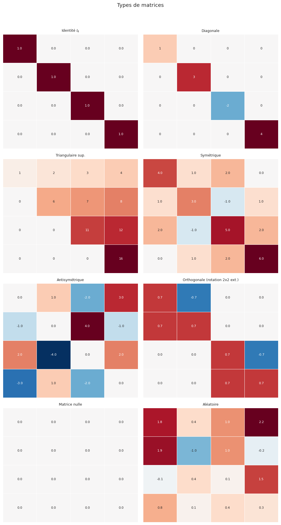
Définition 154 (Matrices particulières)

Nom	Condition
Nulle \(0_{n,p}\)	\(a_{ij} = 0\) pour tout \(i,j\)
Identité \(I_n\)	\(a_{ii} = 1\), \(a_{ij} = 0\) si \(i\neq j\)
Diagonale	\(a_{ij} = 0\) si \(i \neq j\)
Triangulaire sup.	\(a_{ij} = 0\) si \(i > j\)
Triangulaire inf.	\(a_{ij} = 0\) si \(i < j\)
Symétrique	\(A = A^T\)
Antisymétrique	\(A = -A^T\)
Orthogonale	\(A^T A = I_n\) (et \(A \in GL_n(\mathbb{R})\))

_images/0477ba91b25147287bce0a8182f386ee0a12462357530c7861b16458f4f032fd.png

Opérations matricielles#

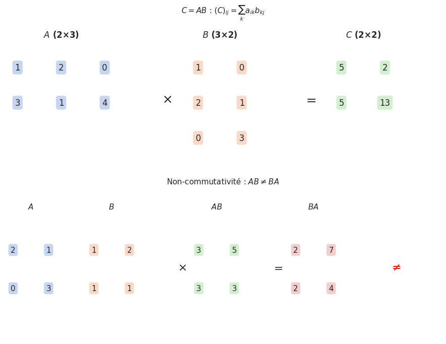
Définition 155 (Produit matriciel)

Le produit \(AB\) de \(A \in \mathcal{M}_{n,p}\) et \(B \in \mathcal{M}_{p,q}\) est la matrice \(C \in \mathcal{M}_{n,q}\) définie par

\[(AB)_{ij} = \sum_{k=1}^{p} a_{ik} b_{kj}.\]

Le coefficient \((i,j)\) est le produit scalaire de la \(i\)-ème ligne de \(A\) par la \(j\)-ème colonne de \(B\).

Proposition 238 (Propriétés du produit)

Associatif : \((AB)C = A(BC)\)
Distributif à gauche et à droite
Élément neutre : \(I_n A = A I_p = A\)
Non commutatif en général : \(AB \neq BA\)
Diviseurs de zéro possibles : \(AB = 0\) n’implique pas \(A = 0\) ou \(B = 0\)

Exemple 83

\(\begin{pmatrix}1&0\\0&0\end{pmatrix}\begin{pmatrix}0&1\\0&0\end{pmatrix} = \begin{pmatrix}0&1\\0&0\end{pmatrix}\) mais \(\begin{pmatrix}0&1\\0&0\end{pmatrix}\begin{pmatrix}1&0\\0&0\end{pmatrix} = \begin{pmatrix}0&0\\0&0\end{pmatrix}\).

Proposition 239 (Transposée)

\((A^T)_{ij} = a_{ji}\). Propriétés :

\((A+B)^T = A^T + B^T\)
\((AB)^T = B^T A^T\)
\((A^T)^T = A\)

_images/56cb472ea126683adb6e53a7d4a0504357243c93bac254526d73ba89c538eb02.png

Matrice d’une application linéaire#

Définition 156 (Matrice d’une application linéaire)

Soit \(\mathcal{B} = (e_1,\ldots,e_n)\) base de \(E\) et \(\mathcal{B}' = (f_1,\ldots,f_p)\) base de \(F\). La matrice de \(f \in \mathcal{L}(E,F)\) dans \((\mathcal{B}, \mathcal{B}')\) est \(A = \mathrm{Mat}_{\mathcal{B},\mathcal{B}'}(f) \in \mathcal{M}_{p,n}(\mathbb{K})\) où la \(j\)-ème colonne contient les coordonnées de \(f(e_j)\) dans \(\mathcal{B}'\) :

\[f(e_j) = \sum_{i=1}^{p} a_{ij} f_i.\]

Proposition 240 (Action par multiplication)

\[[f(u)]_{\mathcal{B}'} = \mathrm{Mat}(f) \cdot [u]_{\mathcal{B}}.\]

L’application \(f \mapsto \mathrm{Mat}(f)\) est un isomorphisme \(\mathcal{L}(E,F) \xrightarrow{\sim} \mathcal{M}_{p,n}(\mathbb{K})\) compatible avec la composition :

\[\mathrm{Mat}(g \circ f) = \mathrm{Mat}(g) \cdot \mathrm{Mat}(f).\]

Exemple 84

Dérivation \(D : \mathbb{R}_3[X] \to \mathbb{R}_3[X]\) dans la base \((1, X, X^2, X^3)\) :

\[\begin{split}\mathrm{Mat}(D) = \begin{pmatrix} 0 & 1 & 0 & 0 \\ 0 & 0 & 2 & 0 \\ 0 & 0 & 0 & 3 \\ 0 & 0 & 0 & 0 \end{pmatrix}.\end{split}\]

C’est une matrice nilpotente : \(\mathrm{Mat}(D)^4 = 0\).

Matrices inversibles et groupe linéaire#

Définition 157 (Matrice inversible)

\(A \in \mathcal{M}_n(\mathbb{K})\) est inversible s’il existe \(B\) tel que \(AB = BA = I_n\). Alors \(B = A^{-1}\) est unique.

L’ensemble \(GL_n(\mathbb{K})\) des matrices inversibles forme un groupe pour le produit (non abélien pour \(n \geq 2\)).

Proposition 241 (Caractérisations de l’inversibilité)

Pour \(A \in \mathcal{M}_n(\mathbb{K})\), les assertions suivantes sont équivalentes :

\(A \in GL_n(\mathbb{K})\)
\(\mathrm{rg}\, A = n\)
\(AX = 0 \Rightarrow X = 0\)
\(\forall B\), le système \(AX = B\) a une unique solution
Les colonnes de \(A\) forment une base de \(\mathbb{K}^n\)
\(\det A \neq 0\) (voir chapitre suivant)

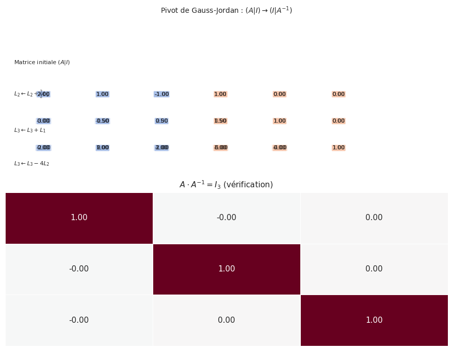
Proposition 242 (Calcul de l’inverse par la méthode de Gauss-Jordan)

On échelonne la matrice augmentée \((A \mid I_n)\) vers \((I_n \mid A^{-1})\) par opérations élémentaires sur les lignes.

_images/0c4dbc101ca9bdd7cff456cc0e6979e9fd8ab004c95c177f5b5fe4d1562f8d4c.png

Systèmes linéaires#

Définition 158 (Système linéaire)

\(AX = B\) avec \(A \in \mathcal{M}_{n,p}\), \(X \in \mathcal{M}_{p,1}\), \(B \in \mathcal{M}_{n,1}\).

Proposition 243 (Structure des solutions)

L’ensemble des solutions de \(AX = B\) est :

\(\emptyset\) si \(\mathrm{rg}(A) \neq \mathrm{rg}(A|B)\) (système incompatible)
\(X_0 + \ker A\) (sous-espace affine de dimension \(p - \mathrm{rg}\, A\)) sinon

où \(X_0\) est une solution particulière quelconque.

Remarque 90

Théorème de Rouché-Fontené. Le système \(AX = B\) est compatible \(\iff\) \(\mathrm{rg}(A) = \mathrm{rg}(A|B)\).

Si compatible, l’ensemble des solutions est un espace affine de dimension \(p - \mathrm{rg}(A)\).

Exemple 85

Pivot de Gauss :

\[\begin{split}\begin{pmatrix}1&2&1\\2&5&3\\1&3&3\end{pmatrix}\begin{pmatrix}x\\y\\z\end{pmatrix} = \begin{pmatrix}4\\10\\7\end{pmatrix}\end{split}\]

Après échelonnement :

\[\begin{split}\begin{pmatrix}1&2&1\\0&1&1\\0&0&1\end{pmatrix}\begin{pmatrix}x\\y\\z\end{pmatrix} = \begin{pmatrix}4\\2\\1\end{pmatrix}\end{split}\]

Remontée : \(z=1\), \(y=1\), \(x=1\). Solution unique \((1,1,1)\).

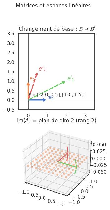
Changement de base#

Définition 159 (Matrice de passage)

La matrice de passage \(P\) de la base \(\mathcal{B}\) à \(\mathcal{B}'\) a pour \(j\)-ème colonne les coordonnées de \(e'_j\) dans \(\mathcal{B}\).

\(P\) est inversible. Si \(X\) et \(X'\) sont les coordonnées d’un même vecteur dans \(\mathcal{B}\) et \(\mathcal{B}'\) :

\[X = PX', \qquad X' = P^{-1}X.\]

Proposition 244 (Formule de changement de base)

\[\mathrm{Mat}_{\mathcal{B}'}(f) = P^{-1} \mathrm{Mat}_{\mathcal{B}}(f) \, P.\]

Définition 160 (Matrices semblables)

\(A\) et \(B\) sont semblables s’il existe \(P \in GL_n\) tel que \(B = P^{-1}AP\).

La semblabilité est une relation d’équivalence. Invariants : rang, trace, déterminant, polynôme caractéristique, valeurs propres.

Trace et invariants#

Définition 161 (Trace)

\(\mathrm{tr}(A) = \sum_{i=1}^n a_{ii}\).

Proposition 245 (Propriétés de la trace)

Linéaire
\(\mathrm{tr}(AB) = \mathrm{tr}(BA)\) (mais \(AB \neq BA\) en général)
\(\mathrm{tr}(P^{-1}AP) = \mathrm{tr}(A)\) (invariant par similitude)

Proof. \(\mathrm{tr}(AB) = \sum_i (AB)_{ii} = \sum_i \sum_k a_{ik}b_{ki} = \sum_k \sum_i b_{ki}a_{ik} = \mathrm{tr}(BA)\).

Opérations élémentaires et pivot de Gauss#

Définition 162 (Matrices élémentaires)

Les opérations élémentaires sur les lignes correspondent à la multiplication à gauche par des matrices inversibles :

Opération	Matrice
\(L_i \leftrightarrow L_j\)	\(E_{ij}\) (permutation)
\(L_i \leftarrow \lambda L_i\)	\(D_i(\lambda)\) (dilatation)
\(L_i \leftarrow L_i + \lambda L_j\)	\(T_{ij}(\lambda)\) (transvection)

Proposition 246 (Forme échelonnée réduite)

Toute matrice \(A\) peut être mise sous forme échelonnée réduite (RREF) par des opérations élémentaires : matrice avec des pivots \(1\) et des zéros au-dessus et en dessous.

La RREF est unique et permet de lire le rang, le noyau, et l’image.

Show code cell source

Hide code cell source

fig, axes = plt.subplots(3, 1, figsize=(9, 11))

# Visualisation du pivot de Gauss (pattern de la matrice augmentée)
np.random.seed(42)
A_rand = np.array([[2., 4., -2., 1.],
                   [1., 3., 4., -2.],
                   [-1., -2., 2., 3.],
                   [3., 6., -1., 4.]])
b = np.array([1., -3., 5., 2.])
Aug_rand = np.hstack([A_rand, b.reshape(-1,1)])

def gauss_elim(M):
    """Retourne la liste des étapes d'élimination."""
    M = M.copy().astype(float)
    steps = [M.copy()]
    n = M.shape[0]
    for col in range(n):
        # Pivot
        pivot_row = col + np.argmax(np.abs(M[col:, col]))
        M[[col, pivot_row]] = M[[pivot_row, col]]
        if abs(M[col, col]) < 1e-12: continue
        for row in range(col+1, n):
            if abs(M[col, col]) > 1e-12:
                M[row] -= (M[row, col]/M[col, col]) * M[col]
        steps.append(M.copy())
    return steps

steps_gauss = gauss_elim(Aug_rand)

for idx, (ax, step, title) in enumerate(zip(
    axes,
    [steps_gauss[0], steps_gauss[2], steps_gauss[-1]],
    ['Matrice initiale $(A|b)$', 'Après 2 pivots', 'Forme échelonnée']
)):
    # Masque de sparsité (zéros vs non-zéros)
    mask_zero = np.abs(step) < 1e-10
    im = ax.imshow(step, cmap='RdBu_r', vmin=-5, vmax=5, aspect='auto')
    for i in range(step.shape[0]):
        for j in range(step.shape[1]):
            val = step[i,j]
            color = 'white' if abs(val) > 2 else 'black'
            ax.text(j, i, f'{val:.1f}', ha='center', va='center',
                    fontsize=9, color=color)
    ax.axvline(3.5, color='orange', lw=2)  # séparation A|b
    ax.set_title(title, fontsize=10)
    ax.set_xticks([]); ax.set_yticks([])

plt.suptitle('Élimination de Gauss : pivot partiel', fontsize=12, y=1.02)
plt.tight_layout()
plt.show()

# Vérification de la solution
A4 = steps_gauss[0][:, :4]
b4 = steps_gauss[0][:, 4]
x_sol = np.linalg.solve(A4, b4)
print(f"Solution : x = {x_sol.round(4)}")
print(f"Vérification Ax = {(A4 @ x_sol).round(4)}, b = {b4.round(4)}")

_images/0d9f98c641eb7318d2c25d1a168896969459c596b9658ebd8761d74080a06bd8.png

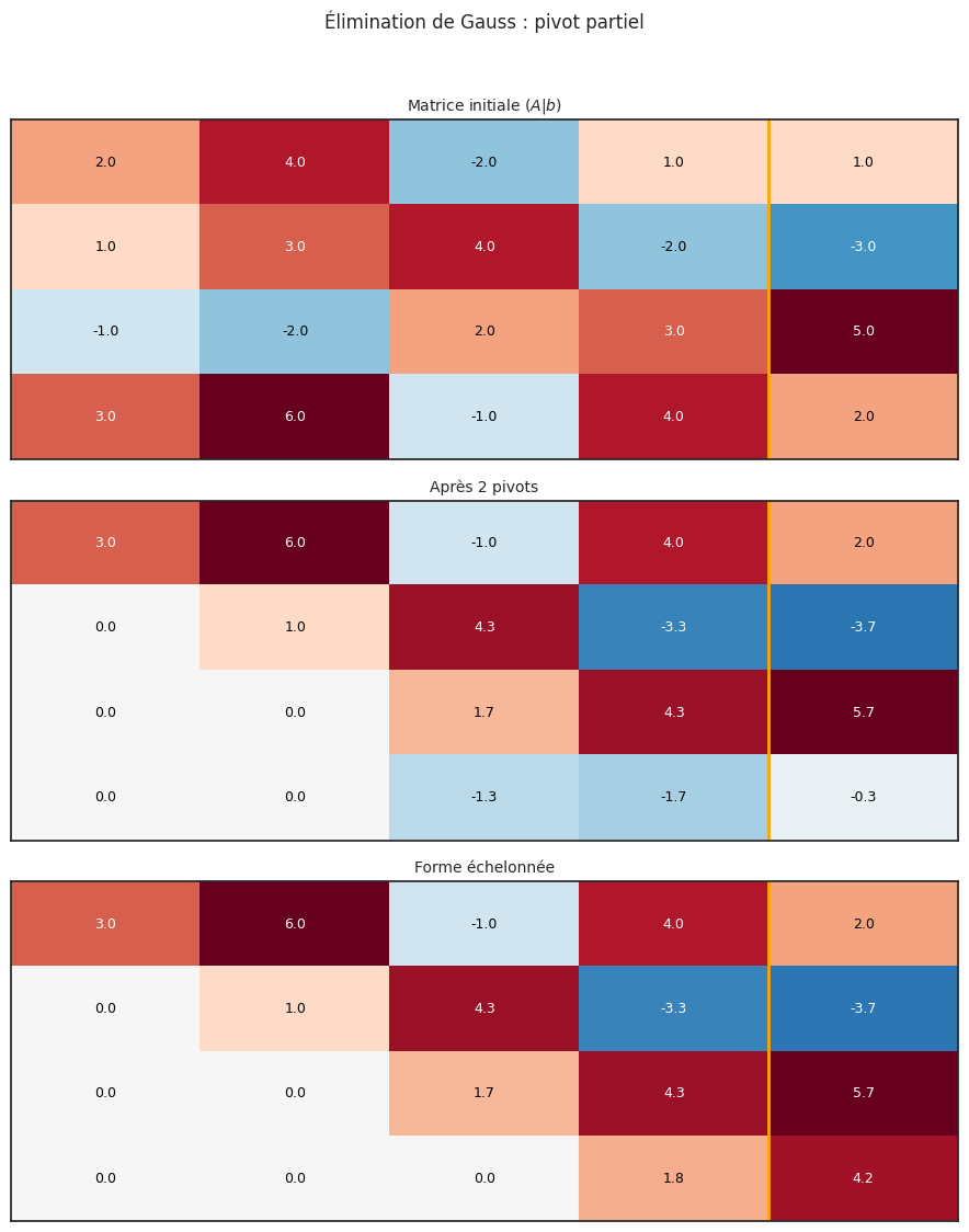
Solution : x = [-34.6667  15.6667  -2.6667   2.3333]
Vérification Ax = [ 1. -3.  5.  2.], b = [ 1. -3.  5.  2.]

Matrices par blocs#

Définition 163 (Matrice par blocs)

Une matrice peut être partitionnée en sous-matrices (blocs) :

\[\begin{split}A = \begin{pmatrix} A_{11} & A_{12} \\ A_{21} & A_{22} \end{pmatrix}.\end{split}\]

Le produit par blocs suit la même règle que le produit matriciel ordinaire, si les dimensions sont compatibles.

Proposition 247 (Inversibilité et blocs diagonaux)

Si \(A = \begin{pmatrix} B & 0 \\ 0 & C \end{pmatrix}\), alors \(A\) est inversible \(\iff\) \(B\) et \(C\) sont inversibles, et \(A^{-1} = \begin{pmatrix} B^{-1} & 0 \\ 0 & C^{-1} \end{pmatrix}\).

Exemple 86

Soit \(A = \begin{pmatrix} 2 & 1 & 0 & 0 \\ 3 & 4 & 0 & 0 \\ 0 & 0 & 1 & 2 \\ 0 & 0 & 3 & 5 \end{pmatrix}\). Alors \(\det A = \det\begin{pmatrix}2&1\\3&4\end{pmatrix} \cdot \det\begin{pmatrix}1&2\\3&5\end{pmatrix} = 5 \cdot (-1) = -5\).

Show code cell source

Hide code cell source

fig, axes = plt.subplots(2, 1, figsize=(9, 7))

# Changement de base : visualisation géométrique
ax = axes[0]
ax.set(xlim=(-0.5, 3.5), ylim=(-0.5, 3.5), aspect='equal',
       title='Changement de base : $\\mathcal{B}$ → $\\mathcal{B}\'$')
ax.axhline(0, color='k', lw=0.5); ax.axvline(0, color='k', lw=0.5)

# Base canonique
for e, c, lbl in [(np.array([1,0]), 'C0', '$e_1$'), (np.array([0,1]), 'C1', '$e_2$')]:
    ax.annotate('', xy=e, xytext=(0,0), arrowprops=dict(arrowstyle='->', color=c, lw=2.5))
    ax.text(e[0]+0.05, e[1]+0.05, lbl, fontsize=12, color=c)

# Nouvelle base B'
e1p = np.array([2, 1]); e2p = np.array([0.5, 1.5])
for e, c, lbl in [(e1p, 'C2', "$e'_1$"), (e2p, 'C3', "$e'_2$")]:
    ax.annotate('', xy=e, xytext=(0,0), arrowprops=dict(arrowstyle='->', color=c, lw=2.5, ls='--'))
    ax.text(e[0]+0.05, e[1]+0.05, lbl, fontsize=12, color=c)

# Matrice de passage
P = np.column_stack([e1p, e2p])
ax.text(1.5, 0.2, f"$P = [[{P[0,0]:.1f}, {P[0,1]:.1f}], [{P[1,0]:.1f}, {P[1,1]:.1f}]]$",
        fontsize=11, ha='center')

# Rang d'une matrice : visualisation
np.random.seed(2)
axes[1].set_title('Rang = nombre de colonnes linéairement indépendantes', fontsize=10)

# Matrice rang 2 dans R^3 : image = plan
v1 = np.array([1,0,0]); v2 = np.array([0,1,0])
# Combinaisons linéaires : nuage de points dans le plan
lambdas = np.linspace(-1, 1, 10)
pts = np.array([a*v1 + b*v2 for a in lambdas for b in lambdas])
ax3d_pos = axes[1].get_position()

ax_3d = fig.add_axes([ax3d_pos.x0, ax3d_pos.y0, ax3d_pos.width, ax3d_pos.height],
                     projection='3d')
axes[1].set_visible(False)
ax_3d.scatter(pts[:,0], pts[:,1], pts[:,2], c='C1', s=15, alpha=0.4)
ax_3d.quiver(0,0,0, v1[0],v1[1],v1[2], color='C2', lw=2, arrow_length_ratio=0.1)
ax_3d.quiver(0,0,0, v2[0],v2[1],v2[2], color='C3', lw=2, arrow_length_ratio=0.1)
ax_3d.set(title='Im($A$) = plan de dim 2 (rang 2)')

plt.suptitle('Matrices et espaces linéaires', fontsize=12, y=1.02)
plt.show()

_images/15869fd35775197e4a3f10719f411ce0bd0aa612c4e3f1e61c6c6735d3cb1441.png