Rétropropagation et optimisation

L’apprentissage n’est rien d’autre que de l’optimisation au service de la généralisation.

Yann LeCun

Le chapitre précédent a introduit le perceptron et les réseaux de neurones multicouches. Mais une question fondamentale demeure : comment ajuster les paramètres d’un réseau pour qu’il résolve la tâche souhaitée ? La réponse tient en deux mots : rétropropagation et optimisation. Ce chapitre développe ces deux piliers, depuis la descente de gradient jusqu’aux algorithmes modernes comme Adam, en passant par le calcul des gradients via la règle de la chaîne, les problèmes de gradients évanescents ou explosifs, la régularisation, l’initialisation des poids, et une implémentation complète en NumPy.

Le problème d’optimisation

Entraîner un réseau de neurones revient à résoudre un problème d’optimisation : trouver les poids \(\boldsymbol{\theta}\) qui minimisent une fonction de coût mesurant l’écart entre prédictions et valeurs attendues.

Définition 204 (Problème d’apprentissage comme optimisation)

Soit \(f_{\boldsymbol{\theta}} : \mathbb{R}^d \to \mathbb{R}^K\) un réseau paramétré par \(\boldsymbol{\theta} \in \mathbb{R}^p\) et \(\{(\mathbf{x}_i, \mathbf{y}_i)\}_{i=1}^n\) un jeu d’entraînement. Le problème s’écrit

\[\min_{\boldsymbol{\theta} \in \mathbb{R}^p} \mathcal{L}(\boldsymbol{\theta}) = \frac{1}{n}\sum_{i=1}^n \ell\bigl(f_{\boldsymbol{\theta}}(\mathbf{x}_i),\, \mathbf{y}_i\bigr)\]

où \(\ell\) est une fonction de perte mesurant l’erreur sur un exemple individuel.

Fonctions de coût classiques

Définition 205 (Erreur quadratique moyenne (MSE))

Pour la régression (\(y_i \in \mathbb{R}\)) : \(\;\mathcal{L}_{\text{MSE}}(\boldsymbol{\theta}) = \frac{1}{n}\sum_{i=1}^n \bigl(f_{\boldsymbol{\theta}}(\mathbf{x}_i) - y_i\bigr)^2\).

Définition 206 (Entropie croisée (cross-entropy))

Pour la classification à \(K\) classes avec sorties softmax \(\hat{\mathbf{y}} = f_{\boldsymbol{\theta}}(\mathbf{x})\) :

\[\mathcal{L}_{\text{CE}}(\boldsymbol{\theta}) = -\frac{1}{n}\sum_{i=1}^n \sum_{k=1}^K y_{ik}\,\log \hat{y}_{ik}\]

où \(y_{ik} = 1\) si l’exemple \(i\) appartient à la classe \(k\) (encodage one-hot). Dans le cas binaire :

\[\mathcal{L}_{\text{BCE}}(\boldsymbol{\theta}) = -\frac{1}{n}\sum_{i=1}^n \bigl[y_i \log \hat{y}_i + (1 - y_i)\log(1 - \hat{y}_i)\bigr]\]

Remarque 175

L’entropie croisée est liée à l’estimation par maximum de vraisemblance. Minimiser \(\mathcal{L}_{\text{CE}}\) revient à maximiser la log-vraisemblance d’un modèle catégoriel. Le choix MSE / cross-entropy n’est pas arbitraire : ce sont les fonctions de coût cohérentes avec les hypothèses distributionnelles (gaussienne / catégorielle).

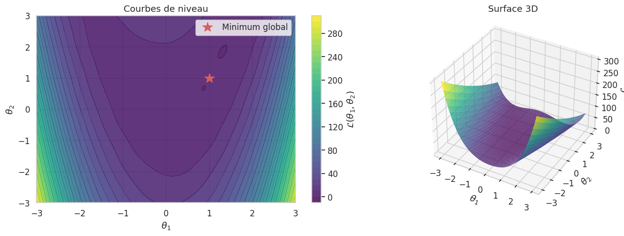
Le paysage de la loss

La fonction \(\mathcal{L}(\boldsymbol{\theta})\) définit une hypersurface dans l’espace des paramètres. Ce paysage est non convexe pour les réseaux de neurones : minima locaux, points-selles et plateaux abondent. Malgré cela, la descente de gradient fonctionne remarquablement bien, car en grande dimension les minima locaux ont généralement des valeurs proches du minimum global.

Show code cell source

Hide code cell source

import numpy as np
import matplotlib.pyplot as plt
import seaborn as sns
from matplotlib import cm

sns.set_theme(style="whitegrid", palette="muted", font_scale=1.1)

Show code cell source

Hide code cell source

# Paysage de loss en 2D
fig = plt.figure(figsize=(14, 5))
theta1 = np.linspace(-3, 3, 200)
theta2 = np.linspace(-3, 3, 200)
T1, T2 = np.meshgrid(theta1, theta2)
L = (1 - T1)**2 + 2*(T2 - T1**2)**2 + 0.3*np.sin(4*T1)*np.sin(4*T2)

ax1 = fig.add_subplot(121)
cp = ax1.contourf(T1, T2, L, levels=30, cmap='viridis', alpha=0.85)
ax1.contour(T1, T2, L, levels=15, colors='k', linewidths=0.3, alpha=0.5)
plt.colorbar(cp, ax=ax1, label='$\\mathcal{L}(\\theta_1, \\theta_2)$')
ax1.plot(1, 1, 'r*', markersize=15, label='Minimum global')
ax1.set_xlabel('$\\theta_1$'); ax1.set_ylabel('$\\theta_2$')
ax1.set_title('Courbes de niveau'); ax1.legend()

ax3d = fig.add_subplot(122, projection='3d')
ax3d.plot_surface(T1, T2, L, cmap='viridis', alpha=0.8, edgecolor='none')
ax3d.set_xlabel('$\\theta_1$'); ax3d.set_ylabel('$\\theta_2$'); ax3d.set_zlabel('$\\mathcal{L}$')
ax3d.set_title('Surface 3D'); ax3d.view_init(elev=35, azim=-60)
plt.tight_layout(); plt.show()

Descente de gradient

La descente de gradient est l’algorithme fondamental pour minimiser \(\mathcal{L}(\boldsymbol{\theta})\). L’idée est simple : à chaque itération, on se déplace dans la direction opposée au gradient, c’est-à-dire dans la direction de plus forte descente locale.

Définition 207 (Descente de gradient)

Soit \(\mathcal{L} : \mathbb{R}^p \to \mathbb{R}\) différentiable. La descente de gradient produit la suite

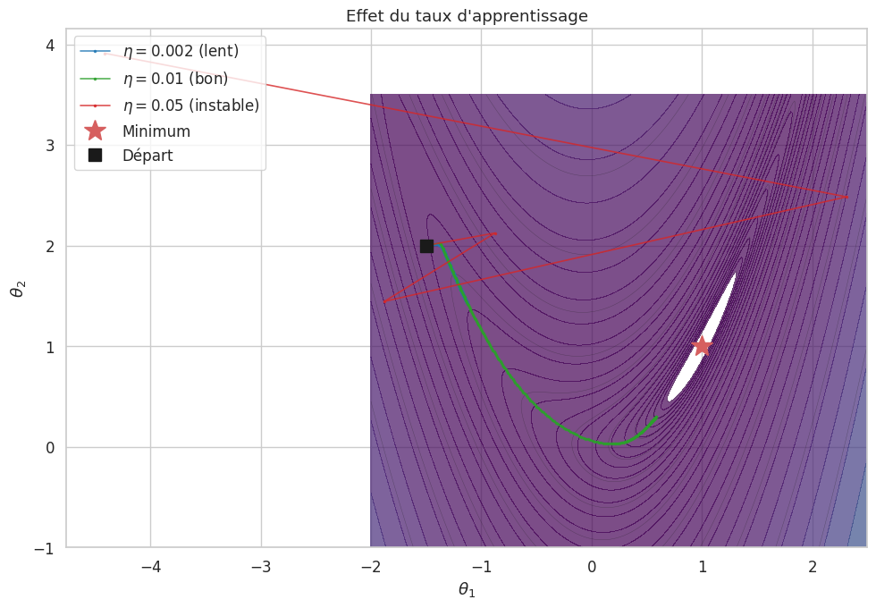
\[\boldsymbol{\theta}^{(t+1)} = \boldsymbol{\theta}^{(t)} - \eta \,\nabla_{\boldsymbol{\theta}}\mathcal{L}(\boldsymbol{\theta}^{(t)})\]

où \(\nabla_{\boldsymbol{\theta}}\mathcal{L}\) est le gradient et \(\eta > 0\) le taux d’apprentissage.

Proposition 55 (Convergence sous convexité)

Si \(\mathcal{L}\) est convexe et \(L\)-lisse (\(\|\nabla\mathcal{L}(\mathbf{a}) - \nabla\mathcal{L}(\mathbf{b})\| \leq L\|\mathbf{a} - \mathbf{b}\|\)), alors pour \(\eta \leq 1/L\) :

\[\mathcal{L}(\boldsymbol{\theta}^{(t)}) - \mathcal{L}(\boldsymbol{\theta}^*) \leq \frac{\|\boldsymbol{\theta}^{(0)} - \boldsymbol{\theta}^*\|^2}{2\eta t}\]

Remarque 176

Le choix de \(\eta\) est crucial : trop grand, l’algorithme diverge ; trop petit, la convergence est lente. En pratique, on utilise un taux adaptatif qui diminue au cours de l’entraînement.

Show code cell source

Hide code cell source

# Descente de gradient sur la fonction de Rosenbrock modifiée
def grad_rosenbrock(theta):
    return np.array([-2*(1-theta[0]) - 20*theta[0]*(theta[1]-theta[0]**2),
                     10*(theta[1]-theta[0]**2)])

def gradient_descent(grad_fn, theta0, lr, n_steps):
    path = [theta0.copy()]
    theta = theta0.copy()
    for _ in range(n_steps):
        g = np.clip(grad_fn(theta), -1e6, 1e6)
        theta = theta - lr * g
        path.append(theta.copy())
    return np.array(path)

theta0 = np.array([-1.5, 2.0])
fig, ax = plt.subplots(figsize=(10, 7))
t1 = np.linspace(-2, 2.5, 300); t2 = np.linspace(-1, 3.5, 300)
T1, T2 = np.meshgrid(t1, t2)
L = (1 - T1)**2 + 5*(T2 - T1**2)**2
ax.contourf(T1, T2, L, levels=np.logspace(-1, 3, 30), cmap='viridis', alpha=0.7)
ax.contour(T1, T2, L, levels=np.logspace(-1, 3, 15), colors='k', linewidths=0.3, alpha=0.4)

for lr, label, c in [(0.002, '$\\eta=0.002$ (lent)', 'tab:blue'),
                      (0.01, '$\\eta=0.01$ (bon)', 'tab:green'),
                      (0.05, '$\\eta=0.05$ (instable)', 'tab:red')]:
    path = gradient_descent(grad_rosenbrock, theta0, lr, 500)
    mask = (np.abs(path[:,0])<5) & (np.abs(path[:,1])<5)
    p = path[mask][:200]
    ax.plot(p[:,0], p[:,1], '-o', color=c, markersize=1.5, linewidth=1.2, label=label, alpha=0.8)

ax.plot(1, 1, 'r*', markersize=18, zorder=5, label='Minimum')
ax.plot(*theta0, 'ks', markersize=10, zorder=5, label='Départ')
ax.set_xlabel('$\\theta_1$'); ax.set_ylabel('$\\theta_2$')
ax.set_title('Effet du taux d\'apprentissage'); ax.legend(loc='upper left')
plt.tight_layout(); plt.show()

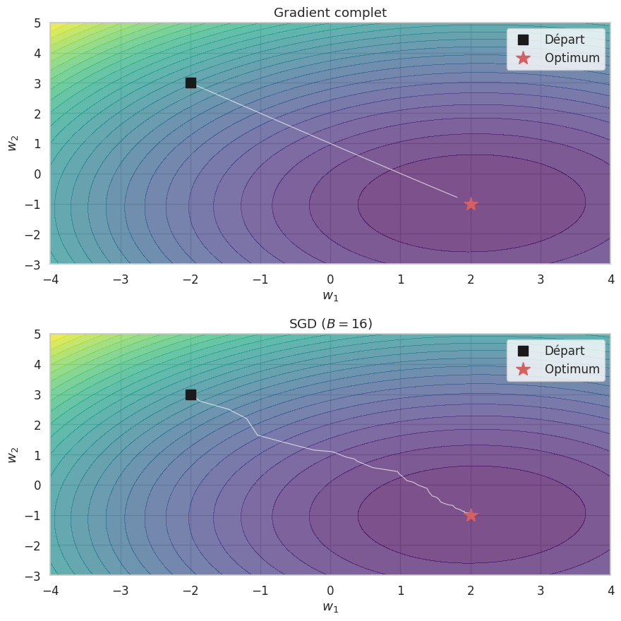
Descente de gradient stochastique (SGD)

Calculer le gradient exact sur tout le jeu de données est prohibitif pour \(n\) grand. La SGD estime le gradient sur un sous-ensemble aléatoire.

Définition 208 (SGD par mini-batches)

À chaque itération, on tire un mini-batch \(\mathcal{B}_t\) de taille \(B\) et on met à jour :

\[\boldsymbol{\theta}^{(t+1)} = \boldsymbol{\theta}^{(t)} - \eta \,\hat{\mathbf{g}}_t, \qquad \hat{\mathbf{g}}_t = \frac{1}{B}\sum_{i \in \mathcal{B}_t} \nabla_{\boldsymbol{\theta}}\,\ell\bigl(f_{\boldsymbol{\theta}^{(t)}}(\mathbf{x}_i),\, \mathbf{y}_i\bigr)\]

L’estimateur \(\hat{\mathbf{g}}_t\) est non biaisé : \(\mathbb{E}[\hat{\mathbf{g}}_t] = \nabla\mathcal{L}(\boldsymbol{\theta}^{(t)})\).

Remarque 177

• \(B = 1\) : SGD pur, très bruité. \(B = n\) : gradient complet, coûteux. \(1 < B < n\) : mini-batch SGD (typiquement \(B \in \{32, 64, 128, 256\}\)).

• Le bruit a un effet régularisant : il aide à échapper aux minima locaux peu profonds.

Définition 209 (Époque)

Une époque = un passage complet sur le jeu d’entraînement, soit \(\lceil n/B \rceil\) itérations.

Show code cell source

Hide code cell source

# Comparaison batch complet vs SGD
np.random.seed(42)
n_samples = 200
X_data = np.random.randn(n_samples, 2)
w_true = np.array([2.0, -1.0])
y_data = X_data @ w_true + 0.3 * np.random.randn(n_samples)

def sgd_path(w0, X, y, lr, batch_size, n_epochs):
    path, w, n = [w0.copy()], w0.copy(), len(y)
    for _ in range(n_epochs):
        for start in range(0, n, batch_size):
            idx = np.random.choice(n, batch_size, replace=False)
            g = 2 * X[idx].T @ (X[idx] @ w - y[idx]) / batch_size
            w = w - lr * g; path.append(w.copy())
    return np.array(path)

w0 = np.array([-2.0, 3.0])
path_full = sgd_path(w0, X_data, y_data, 0.05, n_samples, 30)
path_sgd = sgd_path(w0, X_data, y_data, 0.05, 16, 5)

fig, axes = plt.subplots(2, 1, figsize=(9, 9))
w1r, w2r = np.linspace(-4,4,150), np.linspace(-3,5,150)
W1, W2 = np.meshgrid(w1r, w2r)
L_grid = np.array([[np.mean((X_data@np.array([a,b])-y_data)**2) for a in w1r] for b in w2r])
for ax, path, title in zip(axes, [path_full, path_sgd],
        ['Gradient complet', 'SGD ($B=16$)']):
    ax.contourf(W1, W2, L_grid, levels=30, cmap='viridis', alpha=0.7)
    ax.plot(path[:,0], path[:,1], '-', color='white', linewidth=0.8, alpha=0.7)
    ax.plot(path[0,0], path[0,1], 'ks', markersize=10, label='Départ')
    ax.plot(*w_true, 'r*', markersize=15, label='Optimum')
    ax.set_xlabel('$w_1$'); ax.set_ylabel('$w_2$'); ax.set_title(title); ax.legend()
plt.tight_layout(); plt.show()

La rétropropagation

La SGD requiert \(\nabla_{\boldsymbol{\theta}}\mathcal{L}\). Pour un réseau multicouche, ce calcul repose sur la rétropropagation, application systématique de la règle de la chaîne.

Règle de la chaîne

Proposition 56 (Règle de la chaîne (cas général))

Soient \(\mathbf{g} : \mathbb{R}^m \to \mathbb{R}^n\) et \(\mathbf{f} : \mathbb{R}^n \to \mathbb{R}^p\) différentiables. La jacobienne de \(\mathbf{h} = \mathbf{f} \circ \mathbf{g}\) vérifie

\[\mathbf{J}_{\mathbf{h}}(\mathbf{x}) = \mathbf{J}_{\mathbf{f}}\bigl(\mathbf{g}(\mathbf{x})\bigr) \cdot \mathbf{J}_{\mathbf{g}}(\mathbf{x})\]

Les gradients se propagent de la sortie vers l’entrée (« de droite à gauche »).

Forward et backward pass

Définition 210 (Propagation avant et arrière)

Soit un réseau à \(L\) couches. Le forward pass calcule séquentiellement :

\[\mathbf{z}^{(\ell)} = \mathbf{W}^{(\ell)}\mathbf{a}^{(\ell-1)} + \mathbf{b}^{(\ell)}, \qquad \mathbf{a}^{(\ell)} = \sigma_\ell(\mathbf{z}^{(\ell)}), \qquad \ell = 1, \ldots, L\]

avec \(\mathbf{a}^{(0)} = \mathbf{x}\). Le backward pass calcule le signal d’erreur \(\boldsymbol{\delta}^{(\ell)} = \frac{\partial \mathcal{L}}{\partial \mathbf{z}^{(\ell)}}\) par récurrence :

\[\boldsymbol{\delta}^{(L)} = \frac{\partial \mathcal{L}}{\partial \mathbf{a}^{(L)}} \odot \sigma_L'(\mathbf{z}^{(L)}), \qquad \boldsymbol{\delta}^{(\ell)} = \bigl(\mathbf{W}^{(\ell+1)}\bigr)^T \boldsymbol{\delta}^{(\ell+1)} \odot \sigma_\ell'(\mathbf{z}^{(\ell)})\]

Les gradients des paramètres sont : \(\frac{\partial \mathcal{L}}{\partial \mathbf{W}^{(\ell)}} = \boldsymbol{\delta}^{(\ell)} (\mathbf{a}^{(\ell-1)})^T\) et \(\frac{\partial \mathcal{L}}{\partial \mathbf{b}^{(\ell)}} = \boldsymbol{\delta}^{(\ell)}\).

Calcul détaillé sur un réseau à 2 couches

Exemple 18 (Rétropropagation — réseau à 2 couches)

Architecture : entrée \(\mathbf{x} \in \mathbb{R}^d\), couche cachée (\(h\) neurones, ReLU), sortie scalaire, loss MSE.

Forward : \(\mathbf{z}^{(1)} = \mathbf{W}^{(1)}\mathbf{x} + \mathbf{b}^{(1)}\), \(\mathbf{a}^{(1)} = \text{ReLU}(\mathbf{z}^{(1)})\), \(z^{(2)} = \mathbf{w}^{(2)T}\mathbf{a}^{(1)} + b^{(2)}\), \(\mathcal{L} = (z^{(2)} - y)^2\).

Backward :

1. \(\delta^{(2)} = 2(z^{(2)} - y)\)

2. \(\partial\mathcal{L}/\partial \mathbf{w}^{(2)} = \delta^{(2)} \mathbf{a}^{(1)}\), \(\;\partial\mathcal{L}/\partial b^{(2)} = \delta^{(2)}\)

3. \(\boldsymbol{\delta}^{(1)} = \delta^{(2)} \mathbf{w}^{(2)} \odot \mathbb{1}[\mathbf{z}^{(1)} > 0]\)

4. \(\partial\mathcal{L}/\partial \mathbf{W}^{(1)} = \boldsymbol{\delta}^{(1)} \mathbf{x}^T\), \(\;\partial\mathcal{L}/\partial \mathbf{b}^{(1)} = \boldsymbol{\delta}^{(1)}\)

La complexité est du même ordre que le forward pass.

Remarque 178

La jacobienne de l’activation element-wise est \(\mathbf{J}^{(\ell)} = \text{diag}(\sigma_\ell'(\mathbf{z}^{(\ell)}))\). Le gradient en couche \(\ell\) fait intervenir le produit \(\prod_{k=\ell}^{L} \mathbf{J}^{(k)} \mathbf{W}^{(k)}\) : c’est ce produit itéré qui est à l’origine des problèmes de gradient évanescent ou explosif.

Show code cell source

Hide code cell source

# Forward et backward pass — exemple numérique
np.random.seed(0)
d, h = 3, 4
W1 = np.random.randn(h, d) * 0.5; b1 = np.zeros(h)
w2 = np.random.randn(h) * 0.5; b2 = 0.0
x = np.array([1.0, -0.5, 0.3]); y = 1.5

# Forward
z1 = W1 @ x + b1; a1 = np.maximum(0, z1); z2 = w2 @ a1 + b2; loss = (z2-y)**2
print("=== FORWARD ===")
print(f"z1 = {z1}\na1 = {a1}\nz2 = {z2:.4f},  loss = {loss:.4f}")

# Backward
d2 = 2*(z2-y)
dw2 = d2*a1; db2 = d2
delta1 = (d2*w2) * (z1>0).astype(float)
dW1 = np.outer(delta1, x); db1 = delta1
print("\n=== BACKWARD ===")
print(f"δ₂ = {d2:.4f}\n∂L/∂w₂ = {dw2}\nδ₁ = {delta1}\n∂L/∂W₁ =\n{dW1}")

=== FORWARD ===
z1 = [0.92879757 0.50696542 0.49740068 0.38742938]
a1 = [0.92879757 0.50696542 0.49740068 0.38742938]
z2 = 0.5593,  loss = 0.8849

=== BACKWARD ===
δ₂ = -1.8814
∂L/∂w₂ = [-1.74745077 -0.95381076 -0.93581555 -0.72891424]
δ₁ = [-0.71591271 -0.11446041 -0.41754478 -0.31388942]
∂L/∂W₁ =
[[-0.71591271  0.35795635 -0.21477381]
 [-0.11446041  0.05723021 -0.03433812]
 [-0.41754478  0.20877239 -0.12526343]
 [-0.31388942  0.15694471 -0.09416683]]

Problèmes de gradient

Lorsque les réseaux deviennent profonds (dizaines voire centaines de couches), la rétropropagation se heurte à deux pathologies majeures liées au produit itéré de jacobiens à travers les couches.

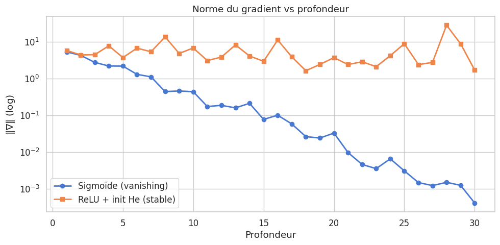
Définition 211 (Gradient évanescent (vanishing gradient))

Si \(\|\mathbf{J}^{(\ell)} \mathbf{W}^{(\ell)}\| < 1\) pour chaque couche, alors \(\|\partial\mathcal{L}/\partial\mathbf{z}^{(1)}\|\) décroît exponentiellement avec la profondeur. Les premières couches cessent d’apprendre.

Définition 212 (Gradient explosif (exploding gradient))

Si \(\|\mathbf{J}^{(\ell)} \mathbf{W}^{(\ell)}\| > 1\), le produit croît exponentiellement : les gradients deviennent gigantesques et l’entraînement diverge.

Remarque 179

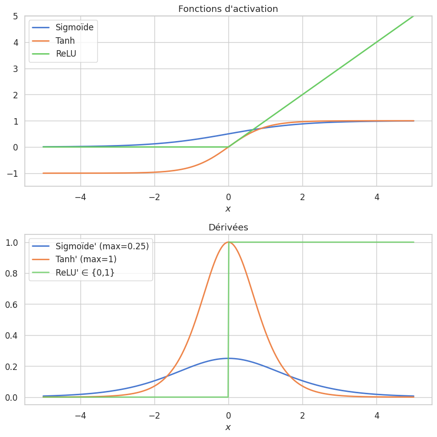
Le rôle de l’activation est central :

• Sigmoïde : \(\sigma'(x) = \sigma(x)(1-\sigma(x)) \leq 0.25\) — vanishing inévitable en profondeur.

• Tanh : \(\tanh'(x) \leq 1\) — mieux, mais encore sensible au vanishing.

• ReLU : \(\text{ReLU}'(x) \in \{0, 1\}\) — préserve l’amplitude du gradient pour les neurones actifs. C’est la raison principale de sa popularité.

Show code cell source

Hide code cell source

# Dérivées des fonctions d'activation
x_act = np.linspace(-5, 5, 500)
sig = 1/(1+np.exp(-x_act)); sig_d = sig*(1-sig)
tanh_v = np.tanh(x_act); tanh_d = 1 - tanh_v**2
relu_d = (x_act > 0).astype(float)

fig, axes = plt.subplots(2, 1, figsize=(9, 9))
axes[0].plot(x_act, sig, lw=2, label='Sigmoïde')
axes[0].plot(x_act, tanh_v, lw=2, label='Tanh')
axes[0].plot(x_act, np.maximum(0, x_act), lw=2, label='ReLU')
axes[0].set_xlabel('$x$'); axes[0].set_title('Fonctions d\'activation')
axes[0].legend(); axes[0].set_ylim(-1.5, 5)

axes[1].plot(x_act, sig_d, lw=2, label="Sigmoïde' (max=0.25)")
axes[1].plot(x_act, tanh_d, lw=2, label="Tanh' (max=1)")
axes[1].plot(x_act, relu_d, lw=2, label="ReLU' ∈ {0,1}", alpha=0.8)
axes[1].set_xlabel('$x$'); axes[1].set_title('Dérivées'); axes[1].legend()
plt.tight_layout(); plt.show()

Show code cell source

Hide code cell source

# Évanouissement du gradient avec la profondeur
np.random.seed(42)
depths = range(1, 31)
norms_sig, norms_relu = [], []
for L in depths:
    g_s, g_r = np.ones(50), np.ones(50)
    for _ in range(L):
        z = np.random.randn(50)
        W_s = np.random.randn(50,50)*0.5; W_r = np.random.randn(50,50)*np.sqrt(2/50)
        g_s = W_s.T @ (g_s * (1/(1+np.exp(-z))) * (1 - 1/(1+np.exp(-z))))
        g_r = W_r.T @ (g_r * (z>0).astype(float))
    norms_sig.append(np.linalg.norm(g_s)); norms_relu.append(np.linalg.norm(g_r))

fig, ax = plt.subplots(figsize=(10, 5))
ax.semilogy(list(depths), norms_sig, 'o-', lw=2, label='Sigmoïde (vanishing)')
ax.semilogy(list(depths), norms_relu, 's-', lw=2, label='ReLU + init He (stable)')
ax.set_xlabel('Profondeur'); ax.set_ylabel('$\\|\\nabla\\|$ (log)')
ax.set_title('Norme du gradient vs profondeur'); ax.legend()
plt.tight_layout(); plt.show()

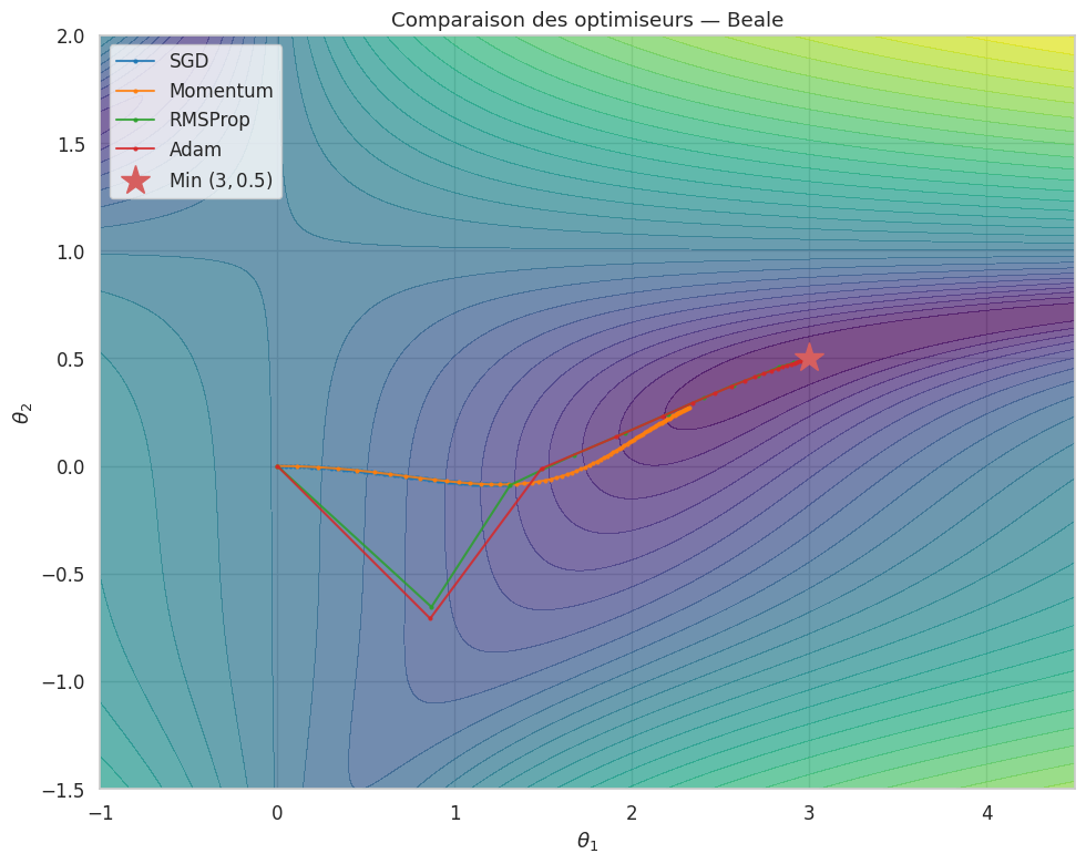
Méthodes d’optimisation avancées

La SGD vanille converge, mais souvent lentement, surtout dans les paysages de loss mal conditionnés (vallées étroites et allongées). Plusieurs variantes améliorent la vitesse et la stabilité de la convergence en modifiant la manière dont les gradients sont accumulés ou normalisés.

Momentum

Définition 213 (SGD avec Momentum)

\[\mathbf{v}^{(t+1)} = \beta\, \mathbf{v}^{(t)} + \nabla\mathcal{L}(\boldsymbol{\theta}^{(t)}), \qquad \boldsymbol{\theta}^{(t+1)} = \boldsymbol{\theta}^{(t)} - \eta\, \mathbf{v}^{(t+1)}\]

où \(\beta \in [0,1)\) (typiquement \(0.9\)). Par analogie physique, \(\mathbf{v}\) est une vitesse et \(\beta\) contrôle la friction.

Momentum de Nesterov

Définition 214 (Nesterov Accelerated Gradient (NAG))

Le gradient est évalué au point « anticipé » \(\boldsymbol{\theta}^{(t)} - \eta\beta\mathbf{v}^{(t)}\) :

\[\mathbf{v}^{(t+1)} = \beta\,\mathbf{v}^{(t)} + \nabla\mathcal{L}\bigl(\boldsymbol{\theta}^{(t)} - \eta\beta\,\mathbf{v}^{(t)}\bigr), \qquad \boldsymbol{\theta}^{(t+1)} = \boldsymbol{\theta}^{(t)} - \eta\,\mathbf{v}^{(t+1)}\]

NAG améliore le taux de convergence de \(O(1/t)\) à \(O(1/t^2)\) sous convexité.

RMSProp

Définition 215 (RMSProp)

Adapte le taux par paramètre via la moyenne mobile des carrés des gradients :

\[\mathbf{s}^{(t+1)} = \rho\,\mathbf{s}^{(t)} + (1-\rho)\,(\nabla\mathcal{L})^2, \qquad \boldsymbol{\theta}^{(t+1)} = \boldsymbol{\theta}^{(t)} - \frac{\eta}{\sqrt{\mathbf{s}^{(t+1)}+\varepsilon}} \odot \nabla\mathcal{L}\]

avec \(\rho = 0.99\), \(\varepsilon = 10^{-8}\). Les directions à grands gradients sont freinées, les autres amplifiées.

Adam

Définition 216 (Adam (Adaptive Moment Estimation))

Adam (Kingma & Ba, 2015) combine Momentum et RMSProp :

\[\mathbf{m}^{(t+1)} = \beta_1 \mathbf{m}^{(t)} + (1-\beta_1)\nabla\mathcal{L}, \qquad \mathbf{v}^{(t+1)} = \beta_2 \mathbf{v}^{(t)} + (1-\beta_2)(\nabla\mathcal{L})^2\]

Correction du biais : \(\hat{\mathbf{m}} = \mathbf{m}/(1-\beta_1^{t+1})\), \(\hat{\mathbf{v}} = \mathbf{v}/(1-\beta_2^{t+1})\).

\[\boldsymbol{\theta}^{(t+1)} = \boldsymbol{\theta}^{(t)} - \frac{\eta}{\sqrt{\hat{\mathbf{v}}}+\varepsilon}\odot\hat{\mathbf{m}}\]

Valeurs par défaut : \(\beta_1=0.9\), \(\beta_2=0.999\), \(\varepsilon=10^{-8}\), \(\eta=10^{-3}\).

Remarque 180

Adam est l’optimiseur le plus utilisé en deep learning grâce à sa robustesse. Cependant, SGD + momentum peut mieux généraliser pour certaines tâches (vision), car Adam converge vers des minima plus « pointus ».

Show code cell source

Hide code cell source

# Comparaison visuelle des optimiseurs sur la fonction de Beale
def grad_beale(theta):
    x, y = theta
    dx = (2*(1.5-x+x*y)*(y-1) + 2*(2.25-x+x*y**2)*(y**2-1)
          + 2*(2.625-x+x*y**3)*(y**3-1))
    dy = (2*(1.5-x+x*y)*x + 2*(2.25-x+x*y**2)*2*x*y
          + 2*(2.625-x+x*y**3)*3*x*y**2)
    return np.array([dx, dy])

def run_optim(grad_fn, theta0, method, lr, n_steps, b1=0.9, b2=0.999, rho=0.99, eps=1e-8):
    theta, path = theta0.copy(), [theta0.copy()]
    m = v = s = np.zeros_like(theta)
    for t in range(1, n_steps+1):
        g = np.clip(grad_fn(theta), -100, 100)
        if method=='sgd': theta = theta - lr*g
        elif method=='momentum': m = b1*m+g; theta = theta - lr*m
        elif method=='rmsprop': s = rho*s+(1-rho)*g**2; theta = theta - lr*g/(np.sqrt(s)+eps)
        elif method=='adam':
            m = b1*m+(1-b1)*g; v = b2*v+(1-b2)*g**2
            theta = theta - lr*(m/(1-b1**t))/(np.sqrt(v/(1-b2**t))+eps)
        path.append(theta.copy())
    return np.array(path)

theta0 = np.array([0.0, 0.0])
opts = {'SGD': run_optim(grad_beale, theta0, 'sgd', 0.00002, 8000),
        'Momentum': run_optim(grad_beale, theta0, 'momentum', 0.00001, 8000),
        'RMSProp': run_optim(grad_beale, theta0, 'rmsprop', 0.005, 8000),
        'Adam': run_optim(grad_beale, theta0, 'adam', 0.01, 8000)}

fig, ax = plt.subplots(figsize=(10, 8))
xr, yr = np.linspace(-1,4.5,300), np.linspace(-1.5,2,300)
Xg, Yg = np.meshgrid(xr, yr)
Zg = np.array([[((1.5-a+a*b)**2+(2.25-a+a*b**2)**2+(2.625-a+a*b**3)**2)
                for a in xr] for b in yr])
ax.contourf(Xg, Yg, np.log1p(Zg), levels=30, cmap='viridis', alpha=0.7)
cols = {'SGD':'tab:blue','Momentum':'tab:orange','RMSProp':'tab:green','Adam':'tab:red'}
for name, path in opts.items():
    mask = (np.abs(path[:,0])<5)&(np.abs(path[:,1])<3); p = path[mask]
    s = max(1,len(p)//80)
    ax.plot(p[::s,0], p[::s,1], '-o', color=cols[name], markersize=2, lw=1.5, label=name, alpha=0.85)
ax.plot(3, 0.5, 'r*', markersize=20, zorder=10, label='Min $(3,0.5)$')
ax.set_xlabel('$\\theta_1$'); ax.set_ylabel('$\\theta_2$')
ax.set_title('Comparaison des optimiseurs — Beale'); ax.legend(loc='upper left')
ax.set_xlim(-1,4.5); ax.set_ylim(-1.5,2); plt.tight_layout(); plt.show()

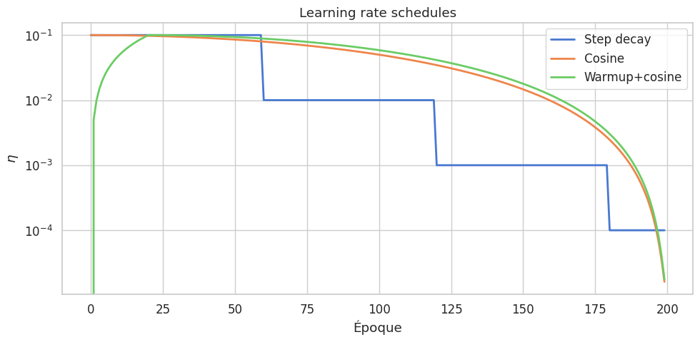
Planification du taux d’apprentissage (learning rate schedules)

Plutôt que d’utiliser un taux constant, on ajuste souvent \(\eta\) au cours de l’entraînement selon un schéma de planification.

Définition 217 (Schémas de planification)

Soit \(\eta_0\) le taux initial, \(T\) le nombre total d’époques.

Step decay : \(\eta_t = \eta_0 \cdot \gamma^{\lfloor t/s \rfloor}\) (\(\gamma=0.1\) typiquement).

Cosine annealing : \(\eta_t = \eta_{\min} + \tfrac{1}{2}(\eta_0 - \eta_{\min})(1 + \cos\tfrac{\pi t}{T})\).

Warmup linéaire : \(\eta_t = \eta_0 \cdot t/T_w\) pour \(t \leq T_w\), puis un autre schéma.

Show code cell source

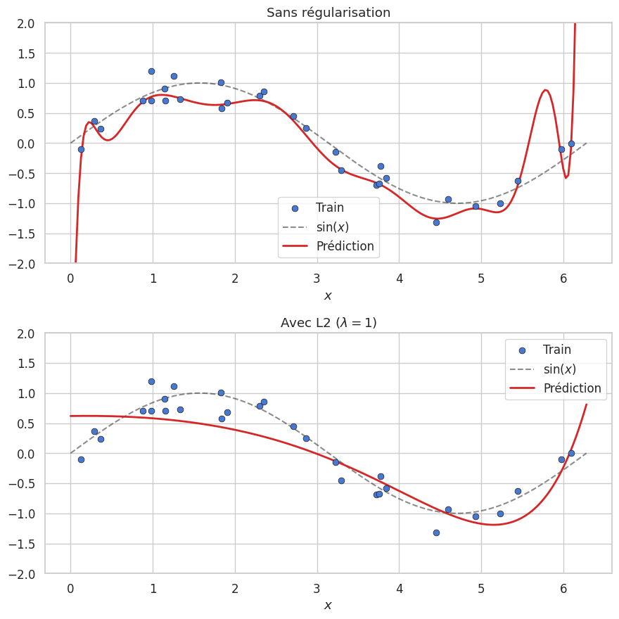
Hide code cell source

T, eta0, eta_min = 200, 0.1, 1e-5
lr_step = [eta0 * 0.1**(t//60) for t in range(T)]
lr_cos = [eta_min + 0.5*(eta0-eta_min)*(1+np.cos(np.pi*t/T)) for t in range(T)]
Tw = 20
lr_wc = [eta0*t/Tw if t<Tw else eta_min+0.5*(eta0-eta_min)*(1+np.cos(np.pi*(t-Tw)/(T-Tw)))
         for t in range(T)]

fig, ax = plt.subplots(figsize=(10, 5))
ax.plot(lr_step, lw=2, label='Step decay'); ax.plot(lr_cos, lw=2, label='Cosine')
ax.plot(lr_wc, lw=2, label='Warmup+cosine')
ax.set_xlabel('Époque'); ax.set_ylabel('$\\eta$'); ax.set_yscale('log')
ax.set_title('Learning rate schedules'); ax.legend()
plt.tight_layout(); plt.show()

Régularisation

La régularisation limite le surapprentissage en contraignant la capacité du modèle.

Définition 218 (Régularisation L2 (weight decay))

\[\widetilde{\mathcal{L}}(\boldsymbol{\theta}) = \mathcal{L}(\boldsymbol{\theta}) + \frac{\lambda}{2}\|\boldsymbol{\theta}\|_2^2\]

La mise à jour devient \(\theta_j \leftarrow (1-\eta\lambda)\theta_j - \eta\,\partial\mathcal{L}/\partial\theta_j\). Le facteur \((1-\eta\lambda)\) « décroît » les poids à chaque étape.

Définition 219 (Dropout)

Pendant l’entraînement, chaque neurone est éteint avec probabilité \(p\) :

\[\tilde{\mathbf{a}}^{(\ell)} = \frac{1}{1-p}\,\mathbf{m}^{(\ell)} \odot \mathbf{a}^{(\ell)}, \qquad m_j \sim \text{Bernoulli}(1-p)\]

Le facteur \(1/(1-p)\) (inverted dropout) assure \(\mathbb{E}[\tilde{\mathbf{a}}] = \mathbf{a}\), évitant toute modification à l’inférence. Le dropout s’interprète comme l’entraînement d’un ensemble exponentiel de sous-réseaux.

Définition 220 (Batch Normalization)

La batch normalization (Ioffe & Szegedy, 2015) normalise les pré-activations sur le mini-batch :

\[\hat{z}_i = \frac{z_i - \mu_{\mathcal{B}}}{\sqrt{\sigma^2_{\mathcal{B}} + \varepsilon}}, \qquad \tilde{z}_i = \gamma\,\hat{z}_i + \beta\]

où \(\gamma, \beta\) sont apprenables. Effets : paysage de loss plus lisse, taux d’apprentissage plus élevés possibles, réduction de la sensibilité à l’initialisation, légère régularisation.

Définition 221 (Early stopping)

On surveille la loss de validation et on arrête l’entraînement lorsqu’elle cesse de diminuer pendant un nombre fixé d’époques (patience). On conserve les poids de la meilleure époque.

Remarque 181

La data augmentation enrichit le jeu d’entraînement par des transformations préservant le label (rotations, retournements, bruit). C’est une régularisation implicite très efficace, surtout en vision.

Show code cell source

Hide code cell source

# Effet de la régularisation L2
np.random.seed(42)
n_train, deg = 30, 15
x_tr = np.sort(np.random.uniform(0, 2*np.pi, n_train))
y_tr = np.sin(x_tr) + 0.2*np.random.randn(n_train)
x_te = np.linspace(0, 2*np.pi, 200); y_te = np.sin(x_te)
Xp = np.column_stack([x_tr**k for k in range(deg+1)])
Xpt = np.column_stack([x_te**k for k in range(deg+1)])
mu, sd = Xp.mean(0), Xp.std(0)+1e-8; Xp_n = (Xp-mu)/sd; Xpt_n = (Xpt-mu)/sd

w_nr = np.linalg.lstsq(Xp_n, y_tr, rcond=None)[0]
w_l2 = np.linalg.solve(Xp_n.T@Xp_n + np.eye(deg+1), Xp_n.T@y_tr)

fig, axes = plt.subplots(2, 1, figsize=(9, 9))
for ax, yp, t in zip(axes, [Xpt_n@w_nr, Xpt_n@w_l2],
        ['Sans régularisation', 'Avec L2 ($\\lambda=1$)']):
    ax.scatter(x_tr, y_tr, s=40, zorder=3, edgecolors='k', lw=0.5, label='Train')
    ax.plot(x_te, y_te, 'k--', lw=1.5, alpha=0.5, label='$\\sin(x)$')
    ax.plot(x_te, np.clip(yp,-3,3), 'tab:red', lw=2, label='Prédiction')
    ax.set_xlabel('$x$'); ax.set_title(t); ax.legend(); ax.set_ylim(-2,2)
plt.tight_layout(); plt.show()

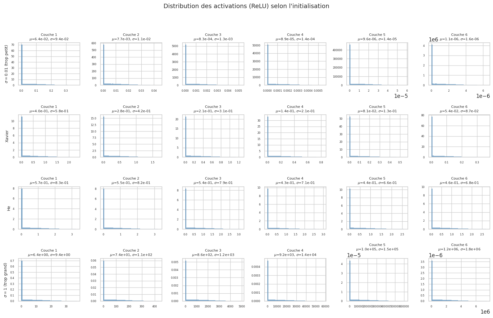
Initialisation des poids

Une mauvaise initialisation conduit immédiatement à des gradients évanescents ou explosifs, avant même le début de l’entraînement.

Proposition 57 (Principe)

Pour qu’un signal se propage correctement, la variance des activations doit rester stable couche après couche. Si les poids sont i.i.d., \(\text{Var}(z_j^{(\ell)}) = n_{\ell-1}\,\text{Var}(W_{ij})\,\text{Var}(a_i^{(\ell-1)})\). La stabilité requiert \(\text{Var}(W_{ij}) \approx 1/n_{\ell-1}\).

Définition 222 (Initialisation Xavier/Glorot)

Pour les activations linéaires ou tanh (Glorot & Bengio, 2010) :

\[W_{ij} \sim \mathcal{N}\!\left(0,\, \frac{2}{n_{\ell-1}+n_\ell}\right) \qquad \text{ou} \qquad W_{ij} \sim \mathcal{U}\!\left(-\sqrt{\frac{6}{n_{\ell-1}+n_\ell}},\, \sqrt{\frac{6}{n_{\ell-1}+n_\ell}}\right)\]

Définition 223 (Initialisation He/Kaiming)

Pour ReLU (He et al., 2015), la moitié des pré-activations étant annulée :

\[W_{ij} \sim \mathcal{N}\!\left(0,\, \frac{2}{n_{\ell-1}}\right)\]

Remarque 182

Xavier et He calibrent la variance des poids pour que le produit itéré de matrices ait des valeurs propres proches de \(1\), stabilisant à la fois le signal (forward) et le gradient (backward).

Show code cell source

Hide code cell source

# Effet de l'initialisation sur les activations à travers les couches
np.random.seed(42)
n_layers, sz, ns = 6, 256, 1000
x0 = np.random.randn(ns, sz)
inits = {'$\\sigma=0.01$ (trop petit)': 0.01, 'Xavier': np.sqrt(1/sz),
         'He': np.sqrt(2/sz), '$\\sigma=1$ (trop grand)': 1.0}

fig, axes = plt.subplots(len(inits), n_layers, figsize=(16, 10))
fig.suptitle('Distribution des activations (ReLU) selon l\'initialisation', fontsize=14, y=1.02)
for row, (name, sigma) in enumerate(inits.items()):
    a = x0.copy()
    for col in range(n_layers):
        a = np.maximum(0, a @ (np.random.randn(sz, sz)*sigma).T)
        ax = axes[row, col]; vals = a.flatten()
        vc = vals[np.abs(vals) < np.percentile(np.abs(vals)+1e-10, 99)]
        if len(vc)>0 and np.std(vc)>1e-10:
            ax.hist(vc, bins=50, density=True, color='steelblue', alpha=0.7, edgecolor='none')
        ax.set_title(f'Couche {col+1}\n$\\mu$={np.mean(a):.1e}, $\\sigma$={np.std(a):.1e}', fontsize=8)
        if col==0: ax.set_ylabel(name, fontsize=9)
        ax.tick_params(labelsize=6)
plt.tight_layout(); plt.show()

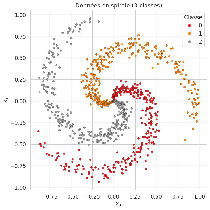
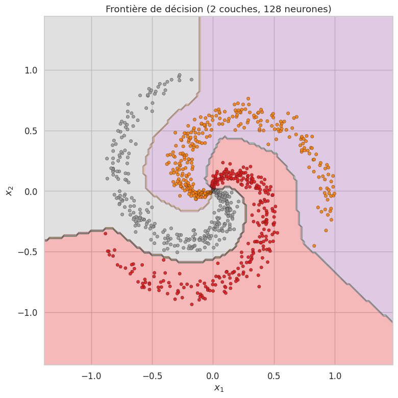
Implémentation from scratch

Mettons en pratique l’ensemble des concepts vus dans ce chapitre en implémentant un réseau de neurones à deux couches entièrement en NumPy, avec forward pass, backward pass (rétropropagation), et entraînement par mini-batch SGD avec l’optimiseur Adam. L’objectif est de classer un jeu de données synthétique non linéairement séparable.

Réseau à 2 couches en NumPy

Show code cell source

Hide code cell source

class NeuralNet2Layers:
    """Réseau 2 couches (1 cachée) en NumPy — forward, backward, Adam."""
    def __init__(self, d_in, d_hid, d_out, lr=0.001):
        self.W1 = np.random.randn(d_in, d_hid)*np.sqrt(2/d_in)
        self.b1 = np.zeros(d_hid)
        self.W2 = np.random.randn(d_hid, d_out)*np.sqrt(1/d_hid)
        self.b2 = np.zeros(d_out)
        self.lr, self.b1_adam, self.b2_adam, self.eps = lr, 0.9, 0.999, 1e-8
        self.t = 0
        self.m = {k: np.zeros_like(v) for k,v in self._p().items()}
        self.v = {k: np.zeros_like(v) for k,v in self._p().items()}
    def _p(self):
        return {'W1':self.W1,'b1':self.b1,'W2':self.W2,'b2':self.b2}
    def forward(self, X):
        self.X = X
        self.z1 = X@self.W1+self.b1; self.a1 = np.maximum(0,self.z1)
        self.z2 = self.a1@self.W2+self.b2; return self.z2
    def softmax(self, z):
        e = np.exp(z-z.max(1,keepdims=True)); return e/e.sum(1,keepdims=True)
    def loss(self, logits, y_oh):
        self.probs = self.softmax(logits)
        return -np.sum(y_oh*np.log(self.probs+1e-12))/y_oh.shape[0]
    def backward(self, y_oh, lam=0.0):
        N = y_oh.shape[0]
        dz2 = (self.probs-y_oh)/N
        self.grads = {
            'W2': self.a1.T@dz2 + lam*self.W2, 'b2': dz2.sum(0),
            'W1': self.X.T@((dz2@self.W2.T)*(self.z1>0).astype(float)) + lam*self.W1,
            'b1': ((dz2@self.W2.T)*(self.z1>0).astype(float)).sum(0)}
    def step(self):
        self.t += 1
        for k in ['W1','b1','W2','b2']:
            g = self.grads[k]
            self.m[k] = self.b1_adam*self.m[k]+(1-self.b1_adam)*g
            self.v[k] = self.b2_adam*self.v[k]+(1-self.b2_adam)*g**2
            mh = self.m[k]/(1-self.b1_adam**self.t)
            vh = self.v[k]/(1-self.b2_adam**self.t)
            upd = self.lr*mh/(np.sqrt(vh)+self.eps)
            if k=='W1': self.W1-=upd
            elif k=='b1': self.b1-=upd
            elif k=='W2': self.W2-=upd
            else: self.b2-=upd
    def predict(self, X):
        return np.argmax(self.forward(X), axis=1)

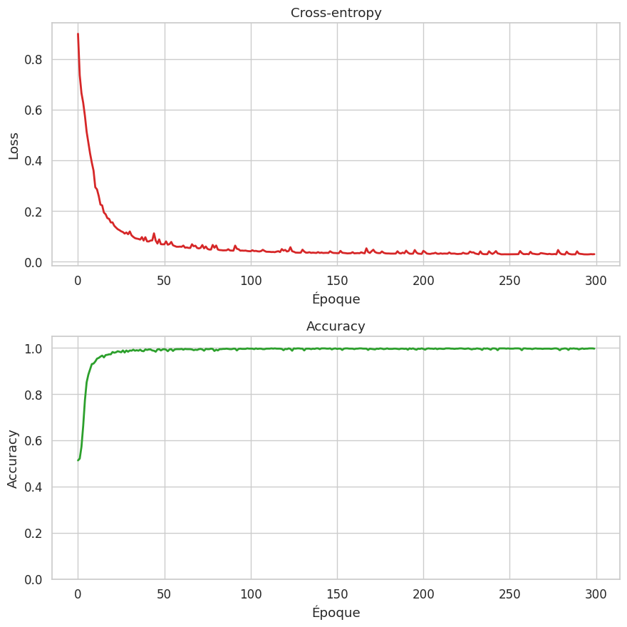
Entraînement sur un jeu synthétique

Show code cell source

Hide code cell source

# Données en spirale (3 classes)
np.random.seed(42)
n_pts, n_cls = 300, 3
X_sp = np.zeros((n_pts*n_cls, 2)); y_sp = np.zeros(n_pts*n_cls, dtype=int)
for k in range(n_cls):
    ix = range(n_pts*k, n_pts*(k+1))
    r = np.linspace(0,1,n_pts)
    th = np.linspace(k*4,(k+1)*4,n_pts)+np.random.randn(n_pts)*0.25
    X_sp[ix] = np.column_stack([r*np.sin(th), r*np.cos(th)]); y_sp[ix] = k
y_oh = np.zeros((len(y_sp), n_cls)); y_oh[np.arange(len(y_sp)), y_sp] = 1

fig, ax = plt.subplots(figsize=(7,7))
sc = ax.scatter(X_sp[:,0], X_sp[:,1], c=y_sp, cmap='Set1', s=20, edgecolors='k', lw=0.3)
ax.set_xlabel('$x_1$'); ax.set_ylabel('$x_2$')
ax.set_title('Données en spirale (3 classes)'); ax.legend(*sc.legend_elements(), title='Classe')
plt.tight_layout(); plt.show()

Show code cell source

Hide code cell source

# Entraînement
net = NeuralNet2Layers(2, 128, 3, lr=0.005)
n_ep, bs = 300, 64; losses, accs = [], []
for ep in range(n_ep):
    perm = np.random.permutation(len(y_sp))
    Xs, ys = X_sp[perm], y_oh[perm]
    ep_loss, nb = 0, 0
    for i in range(0, len(y_sp), bs):
        Xb, yb = Xs[i:i+bs], ys[i:i+bs]
        ep_loss += net.loss(net.forward(Xb), yb); net.backward(yb, lam=1e-4); net.step(); nb+=1
    losses.append(ep_loss/nb); accs.append(np.mean(net.predict(X_sp)==y_sp))
    if (ep+1)%50==0: print(f"Ép. {ep+1:3d} — Loss: {losses[-1]:.4f} — Acc: {accs[-1]:.4f}")
print(f"\nAccuracy finale : {accs[-1]:.4f}")

Ép.  50 — Loss: 0.0686 — Acc: 0.9933
Ép. 100 — Loss: 0.0415 — Acc: 0.9967

Ép. 150 — Loss: 0.0344 — Acc: 0.9978
Ép. 200 — Loss: 0.0308 — Acc: 0.9978

Ép. 250 — Loss: 0.0292 — Acc: 0.9978
Ép. 300 — Loss: 0.0297 — Acc: 0.9967

Accuracy finale : 0.9967

Show code cell source

Hide code cell source

# Courbes d'entraînement
fig, axes = plt.subplots(2, 1, figsize=(9, 9))
axes[0].plot(losses, lw=2, color='tab:red')
axes[0].set_xlabel('Époque'); axes[0].set_ylabel('Loss'); axes[0].set_title('Cross-entropy')
axes[1].plot(accs, lw=2, color='tab:green')
axes[1].set_xlabel('Époque'); axes[1].set_ylabel('Accuracy'); axes[1].set_title('Accuracy')
axes[1].set_ylim(0, 1.05); plt.tight_layout(); plt.show()

Show code cell source

Hide code cell source

# Frontière de décision
h_s = 0.02
xmin, xmax = X_sp[:,0].min()-0.5, X_sp[:,0].max()+0.5
ymin, ymax = X_sp[:,1].min()-0.5, X_sp[:,1].max()+0.5
xx, yy = np.meshgrid(np.arange(xmin,xmax,h_s), np.arange(ymin,ymax,h_s))
Z = net.predict(np.column_stack([xx.ravel(), yy.ravel()])).reshape(xx.shape)

fig, ax = plt.subplots(figsize=(8, 8))
ax.contourf(xx, yy, Z, cmap='Set1', alpha=0.3)
ax.contour(xx, yy, Z, colors='k', linewidths=0.5, alpha=0.3)
ax.scatter(X_sp[:,0], X_sp[:,1], c=y_sp, cmap='Set1', s=20, edgecolors='k', lw=0.3, alpha=0.9)
ax.set_xlabel('$x_1$'); ax.set_ylabel('$x_2$')
ax.set_title('Frontière de décision (2 couches, 128 neurones)')
plt.tight_layout(); plt.show()

Résumé

Ce chapitre a couvert les deux piliers de l’entraînement des réseaux de neurones :

1. La rétropropagation : calcul efficace du gradient via la règle de la chaîne, avec une complexité du même ordre que le forward pass.

2. L’optimisation : de la descente de gradient aux optimiseurs adaptatifs (Adam), en passant par les learning rate schedules et la gestion du bruit stochastique.

Problème	Solutions
Gradient évanescent	ReLU, init He, batch norm, connexions résiduelles
Gradient explosif	Gradient clipping, init soignée, batch norm
Surapprentissage	L2, dropout, early stopping, data augmentation
Convergence lente	Momentum, Adam, LR schedules, warmup
Sensibilité à l’init	Xavier (tanh), He (ReLU), batch norm

En résumé, la rétropropagation fournit un algorithme de calcul des gradients dont la complexité est linéaire en le nombre de paramètres, tandis que les optimiseurs adaptatifs et les techniques de régularisation rendent l’entraînement des réseaux profonds à la fois rapide et robuste. L’ensemble de ces ingrédients — choix de la loss, algorithme d’optimisation, initialisation, régularisation — forme un tout cohérent dont la maîtrise est indispensable pour tout praticien du deep learning.

Le chapitre suivant montrera comment PyTorch automatise la rétropropagation grâce à l”autograd et fournit des implémentations optimisées de l’ensemble des techniques présentées ici, nous permettant de nous concentrer sur l’architecture des réseaux plutôt que sur les calculs de gradient.